Laboratory work in mechanics 1st year. Laboratory works
PREFACE
The publication contains guidelines for performing laboratory work in physics. The description of each work consists of the following parts: title of the work; Objective; instruments and accessories; patterns under study; instructions for making observations; task for processing the results; Control questions.
Job preparation task
When preparing for work, the student must:
1) study the job description and think through answers to security questions;
2) prepare introductory part of the report: title page, title of the work, purpose of the work, description (diagram or sketch) of the laboratory setup and a brief description of the patterns being studied;
3) prepare an observation protocol.
The observation protocol contains: the title of the work; tables that are filled in during the work; information about the student (full name, group number). The form of the tables is developed by the student independently.
Observation protocol and lab report neatly drawn up on one side of A4 paper.
1) title page;
2) introductory part: title of the work, purpose of the work, instruments and accessories, summary of the part of the methodological instructions “research patterns”;
3) calculation part in accordance with the “result processing task”;
4) conclusions from the work.
Calculations must be detailed and provided with the necessary comments. The calculation results, if convenient, are summarized in a table. Drawings and graphs are made in pencil on graph paper.
WORK 1.1. STUDY OF THE MOTION OF BODIES IN A DISSIPATIVE MEDIUM
Devices and accessories: vessel with the test liquid; balls of greater density than the density of the liquid; stopwatch; scale bar.
Purpose of the work: to study the movement of a body in a uniform force field in the presence of environmental resistance and to determine the coefficient of internal friction (viscosity) of the medium.
Patterns under study
Movement of a body in a viscous fluid. A fairly small solid ball falling in a viscous liquid is acted upon by three forces (Fig. 1):
1) gravity mg = 4 3 r 3 πρ g, where r is the radius of the ball; ρ – its density;
2) Archimedes buoyancy force F a = 4 3 r 3 πρ c g , where ρ c is the density of the liquid;
3) medium resistance force (Stokes force)
Fc = 6 πη rv, |
where η is the fluid viscosity coefficient; v is the speed of the ball falling.
Formula (1.1) is applicable to a solid ball moving in a homogeneous liquid at low speed, provided that the distance to the boundaries of the liquid is significantly greater than the diameter of the ball. Resultant force
F = 4 3 r 3 π(ρ−ρc ) g −6 πηrv .
When ρ > ρ c, at the initial stage of movement, while the speed v is small, the ball will fall with acceleration. Upon reaching a certain speed v ∞ at which the resulting

the force becomes zero, the movement of the ball becomes uniform. The speed of uniform motion is determined from the condition F = 0, which gives for v ∞:
v∞ = |
2 r 2 g |
ρ − ρc |
|
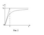
The time dependence of speed v(t) at all stages of movement is described by the expression
v (t ) = v ∞ (1 − e − t τ ) , |
which is obtained after integrating the equation of motion of the ball and substituting the initial conditions. Time τ during which the body could reach a stationary speed v ∞, moving uniformly accelerated with an acceleration equal to the initial
called relaxation time (see Fig. 2). Having experimentally determined the steady-state speed v ∞ of the uniform fall of the ball, we can find the viscosity coefficient of the liquid
η = |
2r 2 (ρ − ρ c )g |
η = |
(1 − |
|||||
3 π Dv∞ |
||||||||
9v∞ |
||||||||
where D is the diameter of the ball, m = π 6 ρ D 3 is its mass.
The viscosity coefficient η is numerically equal to the friction force between adjacent layers of liquid or gas with a unit area of contact between the layers and a unit velocity gradient in the direction perpendicular to the layers. The unit of viscosity is 1 Pa s = 1 N s/m2.
Energy losses in a dissipative system. In steady state, the movement
In this case, the friction force and the force of gravity (taking into account the Archimedes force) are equal to each other and the work of gravity turns completely into heat, and energy dissipation occurs. Energy dissipation rate (power loss) in steady state
find as P ∞ = F 0 v ∞ , where F 0 = m a 0 = m v ∞ / τ ; Thus
P ∞ = m v ∞ 2 / τ .
Instructions for making observations
The body whose motion is being studied is a steel ball (ρ = 7.9.10–3 kg/cm3) of known diameter, and the medium is viscous liquids (various oils). A cylindrical vessel with a scale is filled with liquid, on which two transverse marks are noted at different levels. By measuring the time the ball falls along the path ∆ l from one mark to another, its average speed is found. The found value is the steady-state value of the velocity v ∞ if the distance from the top mark to the liquid level exceeds the relaxation path l τ = v ∞ τ / 2, which is done in this work.
1. Record the diameter of the ball, the density of the liquid under study and the density of the ball material in the observation protocol. Calculate the mass of the ball and record the result in the observation protocol. Prepare 5 balls for measurements.
2. Alternately lowering the balls into the liquid through the inlet pipe with zero initial speed, measure the time with a stopwatch t passing each ball
distances ∆ l between marks in the vessel. Enter the results into the table.
3. Measure the distance ∆ l between the marks. Record the result in the observation protocol.
Results processing task
1. Determination of relaxation time. Using the data obtained, calculate the speed v for each ball. Calculate the initial acceleration using the formula a 0 = g (1 – ρ c / ρ ).
For one of the balls (any one), estimate the relaxation time τ = v ∞ / a 0 . Using formula (1.2) plot the dependence v (t) for the time interval 0< t < 4τ через интервал 0.1 τ . Проанализировать, является ли движение шарика установившимся к моменту прохождения им первой метки, для чего оценить путь релаксации по формуле l τ = v ∞ τ .
2. Energy dissipation assessment. Calculate the power of friction losses in a steady state of motion for the ball, based on the results of observations of the movement of which the relaxation time was determined.

3. Determination of the coefficient of internal friction . Based on the speed of movement of each ball, determine the coefficient of internal friction (η ) liquids. Calculate mean and confidence error∆η .
Control questions
1. What media are called dissipative?
2. Write down the equation of motion of a body in a dissipative medium.
3. What is called relaxation time, and on what parameters of the body and environment does it depend?
4. How does the relaxation time change with a change in the density of the medium?
WORK 2.1. DETERMINATION OF THE MOMENT OF INERTIA OF THE OBERBECK PENDULUM
Devices and accessories: Oberbeck pendulum, set of weights, stopwatch, scale ruler.
Purpose of the work: to study the laws of rotational motion on a cruciform Oberbeck pendulum, to determine the moment of inertia of the pendulum and the moment of friction forces.
The Oberbeck pendulum is a tabletop device (Fig. 1). Three

brackets: top 2, middle 3, bottom 4. The position of all brackets on the vertical stand is strictly fixed. A block 5 is attached to the upper bracket 2 for changing the direction of movement of the thread 6, on which the load 8 is suspended. The rotation of the block 5 is carried out in the bearing assembly 9, which makes it possible to reduce friction. An electromagnet 14 is attached to the middle bracket 3, which, using a friction clutch, when voltage is applied to it, keeps the system with loads stationary. On the same bracket there is a bearing assembly 10, on the axis of which a two-speed pulley 13 is fixed on one side (it has a device for securing the thread 6). At the other end of the axis there is a cross, which consists of four metal rods with marks applied to them every 10 mm and fixed in the boss 12 at right angles to each other. On each rod, weights II can be freely moved and fixed, which makes it possible to stepwise change the moments of inertia of the pendulum cross.
A photoelectric sensor 15 is mounted on the lower bracket 4, which produces an electrical signal to the stopwatch 16 to end the counting of time intervals. A rubber shock absorber 17 is attached to the same bracket, against which the load hits when stopping.
The pendulum is equipped with a 18 mm ruler, which is used to determine the initial and final positions of the weights.
The installation allows for experimental verification of the basic law of the dynamics of rotational motion M = I ε. The pendulum used in this work is a swing
a vik, which is given a cruciform shape (Fig. 2). Loads of mass m f can move along four mutually perpendicular rods. There is a pulley on the common axis; a thread is wound around it, thrown over an additional block, with a set of weights m i tied to its end. Under the action of a falling load m i
the thread unwinds and sets the flywheel into uniformly accelerated motion. The motion of the system is described by the following equations:
mi a = mig – T1 ; |
|
(T 1 – T 2) r 1 – M tr 0 = I 1ε 1, |
|
T 2r 2 – M tr = I 2ε 2; |
where a is the acceleration with which the load is lowered; I 1 – moment of inertia of an additional block with radius r 1; Mtr 0 – moment of friction forces in the axis of the additional block; I 2 – total moment of inertia of the cross with a load, a two-stage pulley and the boss of the cross; Mtr – moment of friction forces in the pulley axis; r 2 – radius of the pulley on which the thread is wound (r 1 = 21 mm, r 2 = 42 mm); ε 1, ε 2 – angular accelerations of the block and
pulley accordingly. Taking into account that ε i = a /r i , from (2.1) we obtain |
|
I 2 = (M – M tr)/ε 2 = (r 2 –M tr)r 2 /a, |
|
where M is the moment of forces applied to the pulley. |
|
If the mass of the additional block is much less than m i, then for small |
|
compared with g values of a, expression (2.2) takes the form |
|
I 2 = (r 2 –M tr)r 2 /a. |
|
If we take into account the moment of forces, friction, acting only on the pulley, then the equation |
|
Relation (2.2) will be written in the form |
|
I 2 = r 2 /a. |
|
where a can be found from the expression S = at 2 /2. |
|
The path length S and the time of lowering the loads t are measured at the installation. Since |
|
Since the moment of friction forces is unknown, then to find I 2 it is advisable to experiment |
|
thoroughly study the dependence of M on ε 2, i.e. |
|
M = I ε 2 + M tr . |
|
Various values of ε 2 are provided by a set of weights m i suspended from the thread.
Thus, having obtained experimental points of the linear dependence of M on ε 2, it is possible, using (2.3), to find both the value of I 2 and M tr. I 2 and Mtr are determined using linear regression formulas (least squares method).
Instructions for making observations
1. Place weights on four mutually perpendicular crosspiece rods at equal distances from the ends of the rods.
Adjust the position of the base using adjusting supports, using a thread with the main weight as a plumb line (the weights should move parallel to the millimeter ruler, descending into the middle of the working window of the photosensor).
3. Rotating the cross counterclockwise, move the main load to the upper position, winding the thread onto a disk of larger radius.
4. Press the “POWER” button located on the front panel of the stopwatch (the lights of the photo sensor and the digital indicators of the stopwatch should light up, as well as the electromagnetic clutch should operate) and fix the crosspiece
V given position.
5. Press the “RESET” button and make sure that the indicators are set to zero.
6. Press the “START” button (the main weight begins to move) and, holding it pressed, make sure that the electromagnet is de-energized, the crosspiece begins to unwind, the stopwatch counts down the time, and at the moment the main weight crosses the optical axis of the photosensor, the time stops. After the time counting stops, return the “START” button
V initial position. In this case, the electromagnetic clutch should operate and slow down the crosspiece.
7. When you press the “START” button, raise the weight to the upper position by winding the thread onto a disk of a larger radius. Return the “START” button to its original position and write down the value of the ruler scale h 1, opposite which is the lower edge of the main
th cargo. The position of the optical axis of the photosensor corresponds to the value h 0 = 495 mm on the ruler scale. Reset the stopwatch indicators by pressing the “RESET” button.
8. Following the instructions in paragraph 6, count the time for lowering the load. Record the results in a table.
9. Measurements according to paragraphs. Do 7 and 8 3 times.
10. Adding additional ones to the main load, measure 3 times for each value of the mass of suspended loads S and t: S = h 0 – h 1.
11. Measurements according to paragraphs. Carry out 8..10, winding the thread onto a disk of smaller radius.
12. Develop the table type yourself.
Results processing tasks
From equation (2.3), using the least squares method (LSM), determine
I 2 and M tr.
a) To do this, using formulas (2.4) and (2.5) for all values of m i and I 2, calculate the values of M k and ε 2 k (18 pairs of values in total);
b) comparing the linear dependence Y = aX + b and equation (2.3), we obtain
X = ε 2, Y = M, a = I 2, b = M tr.
Using the normal linear regression formulas we find , ∆ a and , ∆ b for a given confidence probability.
Using the parameters of the linear dependence found using least squares, construct a graph of the dependence of M on ε 2. Plot the points (ε 2 i , M i ) (i =1..18) on the graph.
Control questions
1. Define angular velocity and angular acceleration.
2. Define and explain the physical meaning of the moment of inertia of point, composite and solid bodies.
3. Write the equation for the dynamics of rotational motion. Indicate in the figure the directions of the vector quantities included in the equation.
4. The moment of inertia of which part of the pendulum is experimentally determined in this work?
5. Derive a formula to calculate the moment of inertia of a pendulum.
6. How will the form of the dependence of angular acceleration on the moment of force change if we assume that there is no friction moment? Draw both dependencies
ε = f(M) on the graph.

WORK 3.1. DETERMINATION OF THE MOMENT OF INERTIA IN THE ATWOOD MACHINE
Devices and accessories: Atwood machine, set of weights, stopwatch, scale ruler.
Purpose of the work: study of rotational and translational movements on the Atwood machine, determination of the moment of inertia of the block and the moment of friction forces in the axis of the block.
Description of the installation and studied patterns
The Atwood machine (Fig. 1) is a tabletop device. On the vertical post 1 of the base 2 there are three brackets: lower 3, middle 4 and upper 5. On the upper bracket 5, a block with a rolling bearing assembly is attached, through which a thread with a load 6 is thrown. On the upper bracket there is an electromagnet 7, which, using a friction clutch, By applying voltage to it, it keeps the system with loads stationary. Photo sensor 8 is mounted on the middle bracket 4, you
giving an electrical signal at the end of counting the time of uniformly accelerated movement of goods. There is a mark on the middle bracket that coincides with the optical axis of the photosensor. The bottom bracket is a platform with a rubber
(All works on mechanics)
Mechanics
No. 1. Physical measurements and calculation of their errors
Familiarization with some methods of physical measurements and calculation of measurement errors using the example of determining the density of a solid body of regular shape.
Download ![]()
No. 2. Determination of the moment of inertia, moment of force and angular acceleration of the Oberbeck pendulum
Determine the moment of inertia of the flywheel (cross with weights); determine the dependence of the moment of inertia on the distribution of masses relative to the axis of rotation; determine the moment of force that causes the flywheel to rotate; determine the corresponding values of angular accelerations.
Download ![]()
No. 3. Determination of the moments of inertia of bodies using a trifilar suspension and verification of Steiner's theorem
Determination of the moments of inertia of some bodies by the method of torsional vibrations using a trifilar suspension; verification of Steiner's theorem.
Download ![]()
No. 5. Determining the speed of a “bullet” by the ballistic method using a unifilar suspension
Determination of the flight speed of a “bullet” using a torsional ballistic pendulum and the phenomenon of absolutely inelastic impact based on the law of conservation of angular momentum
Download ![]()
No. 6. Study of the laws of motion of a universal pendulum
Determination of gravitational acceleration, reduced length, position of the center of gravity and moments of inertia of a universal pendulum.
Download ![]()
No. 9. Maxwell's pendulum. Determination of the moment of inertia of bodies and verification of the law of conservation of energy
Check the law of conservation of energy in mechanics; determine the moment of inertia of the pendulum.
Download ![]()
No. 11. Study of rectilinear uniformly accelerated motion of bodies on the Atwood machine
Determination of free fall acceleration. Determination of the moment of the “effective” resistance force for the movement of loads
Download ![]()
No. 12. Study of the rotational motion of the Oberbeck pendulum
Experimental verification of the basic equation for the dynamics of rotational motion of a rigid body around a fixed axis. Determination of the moments of inertia of the Oberbeck pendulum at various positions of the loads. Determination of the moment of the “effective” resistance force for the movement of loads.
DownloadElectricity
![]()
No. 1. Study of the electrostatic field using modeling method
Constructing a picture of the electrostatic fields of flat and cylindrical capacitors using equipotential surfaces and field lines; comparison of experimental voltage values between one of the capacitor plates and equipotential surfaces with its theoretical values.
Download ![]()
No. 3. Study of the generalized Ohm's law and measurement of electromotive force by the compensation method
Studying the dependence of the potential difference in the section of the circuit containing the EMF on the current strength; calculation of the EMF and impedance of this section.
DownloadMagnetism
![]()
No. 2. Checking Ohm's law for alternating current
Determine the ohmic and inductive resistance of the coil and the capacitive resistance of the capacitor; check Ohm's law for alternating current with different circuit elements
DownloadOscillations and waves
Optics
![]()
No. 3. Determining the wavelength of light using a diffraction grating
Familiarization with a transparent diffraction grating, determining the wavelengths of the spectrum of a light source (incandescent lamp).
DownloadThe quantum physics
![]()
No. 1. Testing black body laws
Study of dependencies: spectral density of energy luminosity of an absolutely black body on the temperature inside the furnace; voltage on the thermocouple from the temperature inside the furnace using a thermocouple.
Materials on the section "Mechanics and Molecular Physics" (1 semester) for 1st year students (1 semester) AVTI, IRE, IET, IEE, InEI (IB)
Materials on the section "Electricity and Magnetism" (2nd semester) for 1st year students (2nd semester) AVTI, IRE, IET, IEE, InEI (IB)
Materials on the section "Optics and Atomic Physics" (3rd semester) for 2nd year students (3rd semester) AVTI, IRE, IET, IEE and 3rd year (5th semester) InEI (IB)
Materials 4th semester
List of laboratory works for the general physics course
Mechanics and molecular physics
1. Errors in physical measurements. Measuring the volume of a cylinder.
2. Determination of the density of the substance and the moments of inertia of the cylinder and ring.
3. Study of conservation laws for collisions of balls.
4. Study of the law of conservation of momentum.
5. Determination of bullet speed using the physical pendulum method.
6. Determination of the average soil resistance force and study of the inelastic collision of a load and a pile using a pile driver model.
7. Study of the dynamics of rotational motion of a rigid body and determination of the moment of inertia of the Oberbeck pendulum.
8. Study of the dynamics of plane motion of the Maxwell pendulum.
9. Determination of the moment of inertia of the flywheel.
10. Determination of the moment of inertia of the pipe and study of Steiner’s theorem.
11. Study of the dynamics of translational and rotational motion using the Atwood device.
12. Determination of the moment of inertia of a flat physical pendulum.
13. Determination of the specific heat of crystallization and the change in entropy during cooling of a tin alloy.
14. Determination of the molar mass of air.
15. Determination of the ratio of heat capacities Cp/Cv of gases.
16. Determination of the mean free path and effective diameter of air molecules.
17. Determination of the coefficient of internal friction of a fluid using the Stokes method.
Electricity and magnetism
1. Study of the electric field using an electrolytic bath.
2. Determination of the electrical capacitance of a capacitor using a ballistic galvanometer.
3. Voltage scales.
4. Determination of the capacitance of a coaxial cable and a parallel-plate capacitor.
5. Study of the dielectric properties of liquids.
6 Determination of the dielectric constant of a liquid dielectric.
7. Study of electromotive force using the compensation method.
8 Determination of magnetic field induction by a measuring generator.
9. Measuring the inductance of the coil system.
10. Study of transient processes in a circuit with inductance.
11. Measurement of mutual inductance.
12. Study of the magnetization curve of iron using the Stoletov method.
13. Familiarization with the oscilloscope and study of the hysteresis loop.
14. Determination of the specific charge of an electron using the magnetron method.
Wave and quantum optics
1. Measuring the wavelength of light using a Fresnel biprism.
2. Determination of the wavelength of light by the Newton ring method.
3. Determination of the wavelength of light using a diffraction grating.
4. Study of diffraction in parallel rays.
5. Study of linear dispersion of a spectral device.
6. Study of Fraunhofer diffraction at one and two slits.
7. Experimental verification of Malu's law.
8. Study of linear emission spectra.
9 Study of the properties of laser radiation.
10 Determination of the excitation potential of atoms using the Frank and Hertz method.
11. Determination of the band gap of silicon based on the red boundary of the internal photoelectric effect.
12 Determination of the red limit of the photoelectric effect and the work function of an electron from a metal.
13. Measuring the temperature of the lamp filament using an optical pyrometer.
Visual physics provides the teacher with the opportunity to find the most interesting and effective teaching methods, making classes interesting and more intense.
The main advantage of visual physics is the ability to demonstrate physical phenomena from a wider perspective and comprehensively study them. Each work covers a large amount of educational material, including from different branches of physics. This provides ample opportunities for consolidating interdisciplinary connections, for generalizing and systematizing theoretical knowledge.
Interactive work in physics should be carried out in lessons in the form of a workshop when explaining new material or when completing the study of a certain topic. Another option is to perform work outside of school hours, in elective, individual classes.
Virtual physics(or physics online) is a new unique direction in the education system. It's no secret that 90% of information enters our brain through the optic nerve. And it is not surprising that until a person sees for himself, he will not be able to clearly understand the nature of certain physical phenomena. Therefore, the learning process must be supported by visual materials. And it’s simply wonderful when you can not only see a static picture depicting any physical phenomenon, but also look at this phenomenon in motion. This resource allows teachers, in an easy and relaxed manner, to clearly demonstrate not only the operation of the basic laws of physics, but will also help conduct online laboratory work in physics in most sections of the general education curriculum. So, for example, how can you explain in words the principle of operation of a pn junction? Only by showing an animation of this process to a child does everything immediately become clear to him. Or you can clearly demonstrate the process of electron transfer when glass rubs on silk, and after that the child will have fewer questions about the nature of this phenomenon. In addition, visual aids cover almost all sections of physics. So for example, want to explain the mechanics? Please, here are animations showing Newton's second law, the law of conservation of momentum when bodies collide, the motion of bodies in a circle under the influence of gravity and elasticity, etc. If you want to study the optics section, nothing could be easier! Experiments on measuring the wavelength of light using a diffraction grating, observation of continuous and line emission spectra, observation of interference and diffraction of light, and many other experiments are clearly shown. What about electricity? And this section is given quite a few visual aids, for example there is experiments to study Ohm's law for complete circuit, mixed conductor connection research, electromagnetic induction, etc.
Thus, the learning process from the “obligatory task” to which we are all accustomed will turn into a game. It will be interesting and fun for the child to look at animations of physical phenomena, and this will not only simplify, but also speed up the learning process. Among other things, it may be possible to give the child even more information than he could receive in the usual form of education. In addition, many animations can completely replace certain laboratory instruments, thus it is ideal for many rural schools, where, unfortunately, even a Brown electrometer is not always available. What can I say, many devices are not even in ordinary schools in large cities. Perhaps by introducing such visual aids into the compulsory education program, after graduating from school we will get people interested in physics, who will eventually become young scientists, some of whom will be able to make great discoveries! In this way, the scientific era of great domestic scientists will be revived and our country will again, as in Soviet times, create unique technologies that are ahead of their time. Therefore, I think it is necessary to popularize such resources as much as possible, to inform about them not only to teachers, but also to schoolchildren themselves, because many of them will be interested in studying physical phenomena not only in lessons at school, but also at home in their free time, and this site gives them such an opportunity! Physics online it's interesting, educational, visual and easily accessible!