What determines the capacity of the valve. Features of the calculation of heating systems with thermostatic valves

kv value.

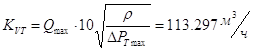
The control valve creates an additional pressure loss in the network to limit the water flow within the required limits. The water flow depends on the differential pressure across the valve:

kv - valve flow rate, ρ - density (for water ρ = 1,000 kg / m 3 at a temperature of 4 ° C, and at 80 ° C ρ = 970 kg / m 3), q - liquid flow rate, m 3 / hour , ∆р – differential pressure, bar.

The maximum value of k v (k vs) is reached when the valve is fully open. This value corresponds to a water flow rate, expressed in m 3 /h, for a differential pressure of 1 bar. The control valve is selected so that the value of kvs provides the design flow for a given differential pressure available when the valve is operated under the given conditions.

It is not easy to determine the value of kvs required for a control valve, since the available differential pressure across the valve depends on many factors:

• Actual pump head.
• Pressure loss in pipes and fittings.
• Pressure loss at terminals.

The pressure loss, in turn, depends on the balancing accuracy.

When designing boiler plants, the theoretically correct values ​​of pressure and flow losses are calculated for various elements of the system. However, in practice, it is rare for different elements to have precisely defined characteristics. During installation, as a rule, pumps, control valves and terminals are selected according to standard characteristics.

Control valves, for example, are produced with values ​​of k vs increasing in geometric proportion, called the Reynard series:

k vs: 1.0 1.6 2.5 4.0 6.3 10 16......

Each value is approximately 60% larger than the previous one.

It is not typical for a control valve to provide exactly the calculated pressure loss for a given flow rate. If, for example, a control valve is to produce a pressure loss of 10 kPa at a given flow rate, then in practice it may be that a valve with a slightly higher kvs value will only create a pressure loss of 4 kPa, while a valve with a slightly lower kvs value will provide a pressure loss. at 26 kPa for the calculated flow rate.

∆p (bar), q (m 3 / h)	∆p (kPa), q (l/s)	∆p (mm BC), q (l/h)	∆p (kPa), q (l/h)
		q = 10k v √∆p	q = 100k v √∆p
	∆p = (36q/kv)2	∆p = (0.1q/kv)2	∆p = (0.01q/kv)2
	kv = 36q/√∆p	k v = 0.1 q/√∆p	kv = 0.01q/√∆p

Some formulas contain consumption, k v and ∆p (ρ = 1,000 kg/m3)

Also, pumps and terminals are often oversized for the same reason. This means that the control valves operate almost closed, and as a result, the regulation cannot be stable. It is also possible that periodically these valves open to the maximum, at start-up necessarily, which leads to excessive flow in this system and insufficient flow in others. As a result, the question should be:

What if the control valve is oversized?

It is clear that, as a rule, it is impossible to accurately select the required control valve.

Consider the case of a 2000 W air heater designed for a temperature drop of 20 K. The pressure loss is 6 kPa for a design flow rate of 2000x0.86/20=86 l/h. If the available differential pressure is 32 kPa and the pressure loss in the pipes and fittings is 4 kPa, a difference of 32 - 6 - 4 = 22 kPa should be across the control valve.

The required value of k vs will be 0.183.

If the minimum available kvs is 0.25, for example, the flow rate instead of the desired 86 l/h will be 104 l/h, an excess of 21%.

In variable flow systems, the differential pressure at the terminals is variable because the pressure loss in the pipes depends on the flow. Control valves are selected for design conditions. At low loads, the maximum potential flow in all installations is increased and there is no danger of excessively low flow in one individual terminal. If maximum load is required under design conditions, it is very important to avoid excess flow.

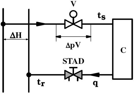
A. Flow limitation by means of a balancing valve installed in series.

If, under design conditions, the flow at the open control valve is higher than the required value, a balancing valve can be installed in series to limit this flow. This will not change the actual control valve control factor, but will even improve its performance (see figure on page 51). The balancing valve is also a diagnostic tool and a shut-off valve.

B. Reduced maximum valve lift.

To compensate for oversized control valve, the degree of opening of the valve can be limited. This solution can be considered for valves with equal percentage characteristics, since the value of k v can be significantly reduced, correspondingly reducing the degree of maximum opening of the valve. If the valve opening degree is reduced by 20%, the maximum value of k v will be reduced by 50%.

In practice, balancing is carried out using balancing valves installed in series with the control valve fully open. Balancing valves are adjusted in each circuit so that at the calculated flow rate, the pressure loss is 3 kPa.

The degree of lift of the control valve is limited when obtained on the balancing valve 3 kPa. Since the plant is balanced and remains balanced, the required flow rate is actually obtained under design conditions.

C. Flow reduction with ∆p regulating valve in the group.

The differential pressure across the control valve can be stabilized as shown in the figure below.

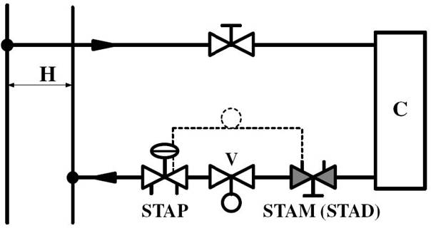
The STAP differential pressure control valve is set to the desired flow rate for a fully open control valve. In this case, the control valve must be exactly sized and its control factor close to one.

A few rules of thumb

If two-way control valves are used in terminals, most of the control valves will be closed or nearly closed at low loads. Since the water flow is low, the pressure loss on pipes and fittings will be negligible. The entire pressure of the pump falls on the control valve, which must be able to resist it. This increase in differential pressure makes it difficult to control at low flow rates, since the actual control factor β" is significantly reduced.

Assume that the control valve is designed for a pressure loss of 4% of the pump head. If the system is running at low flow, the differential pressure is then multiplied by 25. For the same valve opening, the flow is then multiplied by 5 (√25 = 5). The valve is forcibly operated in an almost closed position. This can lead to noise and fluctuations in the setpoint (under these new operating conditions, the valve is oversized by a factor of five).

That is why some authors recommend designing the system in such a way that the calculated pressure drop across the control valves is at least 25% of the pump head. In this case, at low loads, the excess flow on the control valves will not exceed a factor of 2.

It is always very difficult to find a control valve that can withstand such a high differential pressure without making noise. It is also difficult to find sufficiently small valves that meet the above criteria when using low power terminals. In addition, differential pressure variations in the system must be limited, for example by using secondary pumps.

Taking into account this additional concept, the calibration of a two-way control valve must satisfy the following conditions:

• When the system is operating under normal conditions, the flow rate at a fully open valve should be calculated. If the flow is higher than specified, the balancing valve in series should limit the flow. Then for a PI type controller, a control factor of 0.30 will be acceptable. If the control values ​​are lower, the control valve should be replaced with a smaller valve.
• The pump head must be such that the pressure loss across the two-way control valves is at least 25% of the pump head.

For on-off controllers, the concept of control parameters is irrelevant, since the control valve is either open or closed. Therefore, its characteristic does not of great importance. In this case, the flow is slightly limited by the balancing valve installed in series.

(Technical University)

Department of APCP

course project

"Calculation and design of a control valve"

Completed: student gr. 891 Solntsev P.V.

Head: Syagaev N.A.

St. Petersburg 2003

1. Throttle controls

For transportation of liquids and gases in technological processes, as a rule, pressure pipelines are used. In them, the flow moves due to the pressure created by pumps (for liquids) or compressors (for gases). The choice of the required pump or compressor is made according to two parameters: maximum performance and the required pressure.

The maximum performance is determined by the requirements of the technological regulations, the pressure required to ensure maximum flow is calculated according to the laws of hydraulics, based on the length of the route, the number and magnitude of local resistances and the allowable top speed product in the pipeline (for liquids - 2-3 m/s, for gases - 20-30 m/s).

Changing the flow rate in the process pipeline can be done in two ways:

throttling - a change in the hydraulic resistance of the throttle installed on the pipeline (Fig. 1a)

bypassing - changing the hydraulic resistance of the throttle installed on the pipe line connecting the discharge line with the suction line (Fig. 1b)

The choice of how to change the flow rate is determined by the type of pump or compressor used. For the most common pumps and compressors in the industry, both flow control methods can be used.

For positive displacement pumps, such as piston pumps, only liquid bypass is allowed. Throttling the flow for such pumps is unacceptable, because. it can lead to failure of the pump or pipeline.

For reciprocating compressors, both control methods are used.

Changing the flow rate of liquid or gas due to throttling is the main control action in automatic control systems. The throttle used to regulate technological parameters is " regulatory body ».

The main static characteristic of the regulating body is the dependence of the flow through it on the degree of opening:

where q=Q/Q max - relative flow

h=H/H max - the relative stroke of the regulator shutter

This dependency is called consumption characteristic regulatory body. Because The regulating body is a part of the pipeline network, which includes sections of the pipeline, valves, turns and bends of pipes, ascending and descending sections, its flow characteristic reflects the actual behavior of the hydraulic system "regulating body + pipeline network". Therefore, the flow characteristics of two identical regulatory bodies installed on pipelines of different lengths will differ significantly from each other.

Characteristic of the regulatory body, independent of its external connections - " throughput characteristic". This dependence of the relative throughput of the regulatory body s from its relative opening h, i.e.

where: s=K v /K vy is the relative throughput

Other indicators that serve to select a regulatory body are: the diameter of its connecting flanges Du, the maximum allowable pressure Ru, temperature T and the properties of the substance. The index "y" indicates the conditional value of the indicators, which is explained by the inability to ensure their exact observance for serial regulators. Since the flow characteristic of the regulating body depends on the hydraulic resistance of the pipeline network in which it is installed, it is necessary to be able to correct this characteristic. Regulatory bodies that allow such an adjustment are “ control valves". They have solid or hollow cylindrical plungers that allow changing the profile to obtain the required flow characteristic. To facilitate adjustment of the flow characteristic, valves are produced with various types throughput characteristics: linear and equal percentage.

For valves with a linear characteristic, the increase in capacity is proportional to the stroke of the plug, i.e.

where: a is the coefficient of proportionality.

For valves with an equal percentage characteristic, the increase in capacity is proportional to the plunger stroke and the current value of the capacity, i.e.

ds=a*K v *dh (4)

The difference between the throughput and flow characteristics is the greater, the greater the hydraulic resistance of the pipeline network. The ratio of valve capacity to network capacity - the hydraulic module of the system:

n=Kvy/KvT (5)

For values n>1.5 valves with a linear flow characteristic become unusable due to the inconsistency of the proportionality factor a throughout the course. For control valves with an equal percentage flow characteristic, the flow characteristic is close to linear at values n from 1.5 to 6. Since the diameter of the process pipeline Dt is usually chosen with a margin, it may turn out that a control valve with the same or similar nominal diameter Du has excess capacity and, accordingly, the hydraulic module. To reduce the throughput of the valve without changing its connecting dimensions, manufacturers produce valves that differ only in the seat diameter Ds.

2. Assignment for a course project

Option number 7

3. calculation of control valves

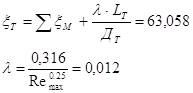
1. Determination of the Reynolds number

, Where - flow rate at maximum flow

r=988.07 kg/m 3 (for water at 50 o C) [table. 2]

m=551*10 -6 Pa*s [table. 3]

Re> 10000, therefore, the flow regime is turbulent.

2. Determination of pressure loss in the pipeline network at maximum flow rate

, Where , x Mvent =4.4, x Mcolen =1.05 [tab. 4]

3. Determination of pressure drop across a control valve at maximum flow rate

4. Determination of the calculated value of the conditional throughput of the control valve:

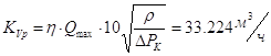, where h=1.25 - safety factor

5. Selection of a control valve with the nearest higher capacity K Vy (according to K Vz and Du):

choose double seated cast iron control valve 25 h30nzhM

conditional pressure 1.6 MPa

conditional pass 50 mm

nominal capacity 40 m3/h

throughput characteristic linear, equal percentage

kind of action BUT

material gray cast iron

medium temperature -15 to +300

6. Determining the capacity of the pipeline network

7. Definition of the hydraulic module of the system

<1.5, следовательно выбираем регулирующий клапан с линейной пропускной характеристикой (ds=a*dh)

Coefficient showing the degree of reduction in the area of ​​the flow section of the valve seat relative to the area of ​​the flow section of the flanges K=0.6 [table. 1]

4. profiling the control valve plunger

The required throughput characteristic of the control valve is ensured by the manufacture of a special shape of the window surface. The optimal plunger profile is obtained by calculating the hydraulic resistance of the throttle pair (plunger - seat) as a function of the relative opening of the control valve.

8. Determination of the coefficient of hydraulic resistance of the valve

, Where , V=2 for double seated valve

9. Determination of the coefficient of hydraulic resistance of the control valve depending on the relative stroke of the plunger

, where h=0.1, 0.2,…,1.0 ,

x dr - coefficient of hydraulic resistance of the throttle pair of the valve x 0 =2.4 [table. 5]

10. According to the schedule in [Fig. 5] the value a k is determined for the relative cross section of the throttle pair

The value of m is specified by the formula:

.

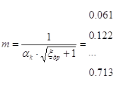The determination of new values ​​of m continues until the new maximum value of m differs from the previous one by less than 5%.

Control valve capacity Kvs- the value of the Kvs coefficient is numerically equal to the water flow through the valve in m³ / h at a temperature of 20 ° C at which the pressure loss on it will be 1 bar. You can calculate the throughput of a control valve for specific system parameters in the Calculations section of the website.

control valve DN- nominal diameter of the hole in the connecting pipes. The DN value is used to unify the standard sizes of pipe fittings. The actual diameter of the hole may slightly differ from the nominal one up or down. An alternative designation for the nominal diameter DN, common in the post-Soviet countries, was the nominal diameter Du of the control valve. A number of conditional passages DN of pipeline fittings is regulated by GOST 28338-89 "Conditional passages (nominal sizes)".

PN control valve- nominal pressure - the highest overpressure of the working medium with a temperature of 20 ° C, at which long-term and safe operation is ensured. An alternative designation for the nominal pressure PN, common in the countries of the post-Soviet space, was the conditional pressure Ru of the valve. A number of nominal pressures PN pipeline fittings are regulated by GOST 26349-84 "Nominal (conditional) pressures".

Dynamic range control, is the ratio of the highest capacity of a fully open control valve (Kvs) to the smallest capacity (Kv) at which the declared flow characteristic is maintained. The dynamic range of control is also called the control ratio.

For example, a valve turndown ratio of 50:1 at Kvs 100 means that the valve can control a flow rate of 2m³/h while maintaining its characteristic flow characteristics.

Most control valves have turndown ratios of 30:1 and 50:1, but there are also very good control valves with a turndown ratio of 100:1.

Control valve authority- characterizes the control ability of the valve. Numerically, the value of authority is equal to the ratio of pressure losses in the fully open valve gate to pressure losses in the regulated section.

The lower the authority of the control valve, the more its flow characteristic deviates from the ideal and the less smooth the change in flow will be when the stem moves. So, for example, in a system controlled by a valve with a linear flow characteristic and low authority, closing the flow section by 50% can reduce the flow by only 10%, while with high authority, closing by 50% should reduce the flow through the valve by 40-50%.

Displays the dependence of the change in the relative flow through the valve on the change in the relative stroke of the control valve stem at a constant pressure drop across it.

Linear flow characteristic- the same increments in the relative stroke of the rod cause the same increments in the relative flow rate. Control valves with a linear flow characteristic are used in systems where there is a direct relationship between the controlled variable and the flow rate of the medium. Control valves with a linear flow characteristic are ideal for maintaining the temperature of the heating medium mixture in substations with dependent connection to the heating network.

Equal percentage flow characteristic(logarithmic) - the dependence of the relative increase in flow rate on the relative increase in the stroke of the rod is logarithmic. Control valves with a logarithmic flow characteristic are used in systems where the controlled variable is non-linearly dependent on the flow through the control valve. So, for example, control valves with an equal percentage flow characteristic are recommended for use in heating systems to control the heat transfer of heating devices, which depends non-linearly on the flow rate of the coolant. Control valves with a logarithmic flow characteristic perfectly regulate the heat transfer of high-speed heat exchangers with a low temperature difference of the coolant. It is recommended to use valves with an equal percentage flow characteristic in systems where a linear flow characteristic is required, and it is not possible to maintain a high authority on the control valve. In this case, the reduced authority distorts the equal percentage characteristic of the valve, bringing it closer to linear. This feature is observed when the authorities of the control valves are not lower than 0.3.

Parabolic flow characteristic- the dependence of the relative increase in flow rate on the relative stroke of the rod obeys a quadratic law (passes along a parabola). Control valves with parabolic flow characteristics are used as a compromise between linear and equal percentage valves.

Specifics of the calculation of a two-way valve

Given:

environment - water, 115C,

∆paccess = 40 kPa (0.4 bar), ∆ppipe = 7 kPa (0.07 bar),

∆pheat exchange = 15 kPa (0.15 bar), nominal flow rate Qnom = 3.5 m3/h,

minimum flow Qmin = 0.4 m3/h

Calculation:

∆paccess = ∆pvalve + ∆ppipe + ∆pheat exchange =
∆pvalve = ∆paccess - ∆ppipe - ∆pheat exchange = 40-7-15 = 18 kPa (0.18 bar)

Safety allowance for working tolerance (provided that the flow rate Q was not overestimated):

Kvs = (1.1 to 1.3). Kv = (1.1 to 1.3) x 8.25 = 9.1 to 10.7 m3/h
From the serially produced series of Kv values, we choose the nearest Kvs value, i.e. Kvs = 10 m3/h. This value corresponds to the clear diameter DN 25. If we select a valve with a threaded connection PN 16 made of gray cast iron, we get the number (order number) of the type:
RV 111 R 2331 16/150-25/T
and corresponding drive.

Determination of the hydraulic loss of a selected and calculated control valve at full opening and a given flow rate.

The actual hydraulic loss of the control valve calculated in this way must be reflected in the hydraulic calculation of the network.

where a must be at least 0.3. The check established: the selection of the valve corresponds to the conditions.

Warning: The calculation of the authority of a two-way control valve is carried out in relation to the differential pressure across the valve in the closed state, i.e. available branch pressure ∆paccess at zero flow, and never relative to the pump pressure ∆ppump, due to the influence of pressure losses in the network pipeline up to the point of connection of the regulated branch. In this case, for convenience, we assume

Regulatory attitude control

Let's carry out the same calculation for the minimum flow rate Qmin = 0.4 m3/h. The minimum flow rate corresponds to pressure drops , , .

Required control ratio

must be less than the set control ratio of the valve r = 50. The calculation satisfies these conditions.

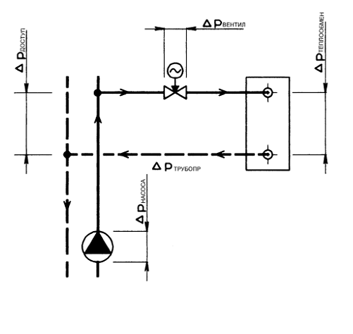
Typical layout of a control loop using a two-way control valve.

Specifics of the calculation of a three-way mixing valve

Given:

environment - water, 90C,

static pressure at connection point 600 kPa (6 bar),

∆ppump2 = 35 kPa (0.35 bar), ∆ppipe = 10 kPa (0.1 bar),

∆pheat exchange = 20 kPa (0.2), nominal flow Qnom = 12 m3/h

Calculation:

Safety allowance for working tolerance (provided that the flow rate Q was not overestimated):
Kvs = (1.1-1.3)xKv = (1.1-1.3)x53.67 = 59.1 to 69.8 m3/h
From a serially produced series of Kv values, we choose the nearest Kvs value, i.e. Kvs = 63 m3/h. This value corresponds to the clear diameter DN65. If we choose flanged ductile iron valve, we get type no.
RV 113 M 6331-16/150-65

We then select the appropriate drive according to the requirements.

Determination of the actual hydraulic loss of the selected valve at full opening

Thus, the calculated actual hydraulic loss of control valves must be reflected in the hydraulic calculation of the network.

Warning: With three-way valves, the most important condition for error-free operation is the minimum differential pressure
on ports A and B. Three-way valves are able to cope with significant differential pressure between ports A and B, but at the cost of a deformation of the control characteristic, and thus a deterioration in the control capacity. Therefore, if there is even the slightest doubt about the pressure difference between the two connections (for example, if a three-way valve without a pressure compartment is directly connected to the primary network), we recommend using a two-way valve in connection with a hard circuit for good control.

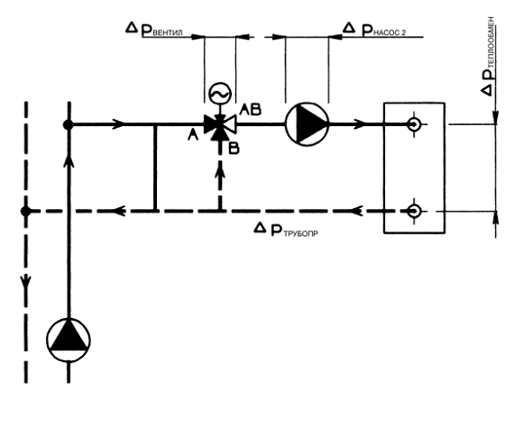
Typical control line layout using a three-way mixing valve.

There is an opinion that the selection of a three-way valve does not require preliminary calculations. This opinion is based on the assumption that the total flow through the branch pipe AB - does not depend on the stroke of the rod and is always constant. In fact, the flow through the common port AB fluctuates depending on the stroke of the stem, and the amplitude of the oscillation depends on the authority of the three-way valve in the regulated area and its flow characteristics.

Method for calculating a three-way valve

Three-way valve calculation perform in the following sequence:

• 1. Selection of the optimal flow characteristics.
• 2. Determination of the control capacity (valve authority).
• 3. Determination of throughput and nominal diameter.
• 4. Selection of the control valve electric drive.
• 5. Check for noise and cavitation.

Flow characteristics selection

The dependence of the flow through the valve on the stroke of the stem is called the flow characteristic. The type of flow characteristic determines the shape of the plug and valve seat. Since the three-way valve has two gates and two seats, it also has two flow characteristics, the first is the characteristic along the straight stroke - (A-AB), and the second along the perpendicular - (B-AB).

Linear/Linear. The total flow through the branch pipe AB is constant only when the valve authority is equal to 1, which is practically impossible to ensure. Operating a three-way valve with an authority of 0.1 will result in fluctuations in the total flow during stem movement, ranging from 100% to 180%. Therefore, valves with a linear/linear characteristic are used in systems that are insensitive to flow fluctuations, or in systems with a valve authority of at least 0.8.

logarithmic/logarithmic. The minimum fluctuations in the total flow through the branch pipe AB in three-way valves with a logarithmic / logarithmic flow characteristic are observed at a valve authority of 0.2. At the same time, a decrease in authority, relative to the specified value, increases, and an increase - reduces the total flow through the branch pipe AB. The fluctuation of the flow rate in the range of authorities from 0.1 to 1 is from +15% to -55%.

log/linear. Three-way valves with a logarithmic/linear flow characteristic are used if the circulation rings passing through the A-AB and B-AB connections require regulation according to different laws. Flow stabilization during the movement of the valve stem occurs at an authority equal to 0.4. The fluctuation of the total flow through the branch pipe AB in the range of authorities from 0.1 to 1 is from +50% to -30%. Control valves with a logarithmic / linear flow characteristic are widely used in control units for heating systems and heat exchangers.

Authority calculation

Authority of the three-way valve is equal to the ratio of pressure loss on the valve to the pressure loss on the valve and the regulated section. The authority value for three-way valves determines the range of fluctuation in the total flow through port AB.

A 10% deviation of the instantaneous flow rate through port AB during stroke is provided at the following authority values:

• A+ = (0.8-1.0) - for a linear/linear valve.
• A+ = (0.3-0.5) - for a valve with a logarithmic / linear characteristic.
• A+ = (0.1-0.2) - for a valve with a logarithmic / logarithmic characteristic.

Bandwidth calculation

The dependence of pressure loss on the valve from the flow through it is characterized by the Kvs capacity factor. The Kvs value is numerically equal to the flow in m³/h through a fully open valve, at which the pressure loss on it is 1 bar. As a rule, the Kvs value of a three-way valve is the same for the A-AB and B-AB strokes, but there are valves with different capacities for each of the strokes.

Knowing that when the flow rate changes by “n” times, the head loss on the valve changes by “n²” times, it is not difficult to determine the required Kvs of the control valve by substituting the calculated flow rate and head loss into the equation. From the nomenclature, a three-way valve is selected with the closest value of the throughput coefficient to the value obtained as a result of the calculation.

Selection of an electric drive

The electric actuator is matched to the previously selected three-way valve. Electric actuators are recommended to be selected from the list of compatible devices specified in the valve specifications, while paying attention to:

• The actuator and valve interfaces must be compatible.
• The stroke of the electric actuator must be at least the stroke of the valve stem.
• Depending on the inertia of the regulated system, drives with different speeds of action should be used.
• The closing force of the actuator determines the maximum differential pressure across the valve at which the actuator can close it.
• One and the same electric actuator ensures the closing of a three-way valve working for mixing and flow separation, at different pressure drops.
• The supply voltage and control signal of the drive must match the supply voltage and control signal of the controller.
• Rotary three-way valves are used with rotary, and saddle valves with linear electric drives.

Calculation for the possibility of cavitation

Cavitation is the formation of steam bubbles in a water stream, which manifests itself when the pressure in it decreases below the saturation pressure of water vapor. The Bernoulli equation describes the effect of increasing the flow velocity and reducing the pressure in it, which occurs when the flow section narrows. The flow area between the shutter and the three-way valve seat is the very narrowing, the pressure in which can drop to saturation pressure, and the place where cavitation is most likely to occur. Vapor bubbles are unstable, they appear sharply and also collapse sharply, this leads to metal particles being eaten out of the valve shutter, which will inevitably cause premature wear. In addition to wear, cavitation leads to increased noise during valve operation.

The main factors affecting the occurrence of cavitation:

• Water temperature - the higher it is, the greater the likelihood of cavitation.


• Water pressure - in front of the control valve, the higher it is, the less likely it is to cause cavitation.


• Permissible pressure losses - the higher they are, the higher the likelihood of cavitation. It should be noted here that in the valve position close to closing, the throttled pressure on the valve tends to the available pressure in the regulated area.


• The cavitation characteristic of a three-way valve is determined by the characteristics of the throttling element of the valve. The cavitation coefficient is different for different types of control valves and should be specified in their technical characteristics, but since most manufacturers do not specify this value, the calculation algorithm includes a range of the most probable cavitation coefficients.

As a result of the cavitation test, the following result can be produced:

• "No" - there will definitely be no cavitation.
• "Possible" - cavitation may occur on valves of some designs, it is recommended to change one of the above-described influence factors.
• "Yes" - cavitation will definitely be, change one of the factors influencing the occurrence of cavitation.

Noise calculation

A high flow rate at the inlet of a three-way valve can cause high noise levels. For most rooms where control valves are installed, the permissible noise level is 35-40 dB(A) which corresponds to a velocity in the valve inlet of about 3m/s. Therefore, when selecting a three-way valve, it is not recommended to exceed the specified speed.