Linear inequalities. Systems of linear inequalities

see also Solving a linear programming problem graphically, Canonical form of linear programming problems

The system of constraints for such a problem consists of inequalities in two variables:
and the objective function has the form F = C 1 x + C 2 y which needs to be maximized.

Let's answer the question: what pairs of numbers ( x; y) are solutions to the system of inequalities, i.e., satisfy each of the inequalities simultaneously? In other words, what does it mean to solve a system graphically?
First you need to understand what is the solution to one linear inequality with two unknowns.
Solving a linear inequality with two unknowns means determining all pairs of unknown values ​​for which the inequality holds.
For example, inequality 3 x – 5y≥ 42 satisfy pairs ( x , y) : (100, 2); (3, –10), etc. The task is to find all such pairs.
Let's consider two inequalities: ax + by≤ c, ax + by≥ c. Straight ax + by = c divides the plane into two half-planes so that the coordinates of the points of one of them satisfy the inequality ax + by >c, and the other inequality ax + +by <c.
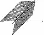
Indeed, let us take a point with coordinate x = x 0 ; then a point lying on a line and having an abscissa x 0, has an ordinate

Let for certainty a< 0, b>0, c>0. All points with abscissa x 0 lying above P(for example, dot M), have y M>y 0 , and all points below the point P, with abscissa x 0 , have y N<y 0 . Because the x 0 is an arbitrary point, then there will always be points on one side of the line for which ax+ by > c, forming a half-plane, and on the other side - points for which ax + by< c.

Picture 1

The inequality sign in the half-plane depends on the numbers a, b , c.
This implies the following method for graphically solving systems of linear inequalities in two variables. To solve the system you need:

1. For each inequality, write the equation corresponding to this inequality.
2. Construct straight lines that are graphs of functions specified by equations.
3. For each line, determine the half-plane, which is given by the inequality. To do this, take an arbitrary point that does not lie on a line and substitute its coordinates into the inequality. if the inequality is true, then the half-plane containing the chosen point is the solution to the original inequality. If the inequality is false, then the half-plane on the other side of the line is the set of solutions to this inequality.
4. To solve a system of inequalities, it is necessary to find the area of ​​intersection of all half-planes that are the solution to each inequality of the system.

This area may turn out to be empty, then the system of inequalities has no solutions and is inconsistent. Otherwise, the system is said to be consistent.
There can be a finite number or an infinite number of solutions. The area can be a closed polygon or unbounded.

Let's look at three relevant examples.

Example 1. Solve the system graphically:
x + y – 1 ≤ 0;
–2x – 2y + 5 ≤ 0.

• consider the equations x+y–1=0 and –2x–2y+5=0 corresponding to the inequalities;
• Let's construct straight lines given by these equations.

Figure 2

Let us define the half-planes defined by the inequalities. Let's take an arbitrary point, let (0; 0). Let's consider x+ y– 1 0, substitute the point (0; 0): 0 + 0 – 1 ≤ 0. This means that in the half-plane where the point (0; 0) lies, x + y – 1 ≤ 0, i.e. the half-plane lying below the line is a solution to the first inequality. Substituting this point (0; 0) into the second, we get: –2 ∙ 0 – 2 ∙ 0 + 5 ≤ 0, i.e. in the half-plane where the point (0; 0) lies, –2 x – 2y+ 5≥ 0, and we were asked where –2 x – 2y+ 5 ≤ 0, therefore, in the other half-plane - in the one above the straight line.
Let's find the intersection of these two half-planes. The lines are parallel, so the planes do not intersect anywhere, which means that the system of these inequalities has no solutions and is inconsistent.

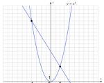
Example 2. Find graphically solutions to the system of inequalities:

Figure 3
1. Let's write out the equations corresponding to the inequalities and construct straight lines.
x + 2y– 2 = 0

x	2	0
y	0	1

y – x – 1 = 0

x	0	2
y	1	3

y + 2 = 0;
y = –2.
2. Having chosen the point (0; 0), we determine the signs of inequalities in the half-planes:
0 + 2 ∙ 0 – 2 ≤ 0, i.e. x + 2y– 2 ≤ 0 in the half-plane below the straight line;
0 – 0 – 1 ≤ 0, i.e. y –x– 1 ≤ 0 in the half-plane below the straight line;
0 + 2 =2 ≥ 0, i.e. y+ 2 ≥ 0 in the half-plane above the straight line.
3. The intersection of these three half-planes will be an area that is a triangle. It is not difficult to find the vertices of the region as the intersection points of the corresponding lines


Thus, A(–3; –2), IN(0; 1), WITH(6; –2).

Let's consider another example in which the resulting solution domain of the system is not limited.

Maintaining your privacy is important to us. For this reason, we have developed a Privacy Policy that describes how we use and store your information. Please review our privacy practices and let us know if you have any questions.

Collection and use of personal information

Personal information refers to data that can be used to identify or contact a specific person.

You may be asked to provide your personal information at any time when you contact us.

Below are some examples of the types of personal information we may collect and how we may use such information.

What personal information do we collect:

• When you submit an application on the site, we may collect various information, including your name, telephone number, email address, etc.

How we use your personal information:

• The personal information we collect allows us to contact you with unique offers, promotions and other events and upcoming events.
• From time to time, we may use your personal information to send important notices and communications.
• We may also use personal information for internal purposes, such as conducting audits, data analysis and various research in order to improve the services we provide and provide you with recommendations regarding our services.
• If you participate in a prize draw, contest or similar promotion, we may use the information you provide to administer such programs.

Disclosure of information to third parties

We do not disclose the information received from you to third parties.

Exceptions:

• If necessary - in accordance with the law, judicial procedure, in legal proceedings, and/or on the basis of public requests or requests from government bodies in the Russian Federation - to disclose your personal information. We may also disclose information about you if we determine that such disclosure is necessary or appropriate for security, law enforcement, or other public importance purposes.
• In the event of a reorganization, merger, or sale, we may transfer the personal information we collect to the applicable successor third party.

Protection of personal information

We take precautions - including administrative, technical and physical - to protect your personal information from loss, theft, and misuse, as well as unauthorized access, disclosure, alteration and destruction.

Respecting your privacy at the company level

To ensure that your personal information is secure, we communicate privacy and security standards to our employees and strictly enforce privacy practices.

There are only “X’s” and only the abscissa axis, but now “Y’s” are added and the field of activity expands to the entire coordinate plane. Further in the text, the phrase “linear inequality” is understood in a two-dimensional sense, which will become clear in a matter of seconds.

In addition to analytical geometry, the material is relevant for a number of problems in mathematical analysis and economic and mathematical modeling, so I recommend studying this lecture with all seriousness.

Linear inequalities

There are two types of linear inequalities:

1) Strict inequalities: .

2) Lax inequalities: .

What is the geometric meaning of these inequalities? If a linear equation defines a line, then a linear inequality defines half-plane.

To understand the following information, you need to know the types of lines on a plane and be able to construct straight lines. If you have any difficulties in this part, read the help Graphs and properties of functions– paragraph about linear function.

Let's start with the simplest linear inequalities. The dream of every poor student is a coordinate plane on which there is nothing:

As you know, the x-axis is given by the equation - the “y” is always (for any value of “x”) equal to zero

Let's consider inequality. How to understand it informally? “Y” is always (for any value of “x”) positive. Obviously, this inequality defines the upper half-plane - after all, all the points with positive “games” are located there.

In the event that the inequality is not strict, to the upper half-plane additionally the axis itself is added.

Similarly: the inequality is satisfied by all points of the lower half-plane; a non-strict inequality corresponds to the lower half-plane + axis.

The same prosaic story is with the y-axis:

– the inequality specifies the right half-plane;
– the inequality specifies the right half-plane, including the ordinate axis;
– the inequality specifies the left half-plane;
– the inequality specifies the left half-plane, including the ordinate axis.

In the second step, we consider inequalities in which one of the variables is missing.

Missing "Y":

Or there is no “x”:

These inequalities can be dealt with in two ways: please consider both approaches. Along the way, let’s remember and consolidate school actions with inequalities, already discussed in class Function Domain.

Example 1

Solve linear inequalities:

What does it mean to solve a linear inequality?

Solving a linear inequality means finding a half-plane, whose points satisfy this inequality (plus the line itself, if the inequality is not strict). Solution, usually, graphic.

It’s more convenient to immediately execute the drawing and then comment out everything:

a) Solve the inequality

Method one

The method is very reminiscent of the story with coordinate axes, which we discussed above. The idea is to transform the inequality - to leave one variable on the left side without any constants, in this case the variable “x”.

Rule: In an inequality, the terms are transferred from part to part with a change of sign, while the sign of the inequality ITSELF does not change(for example, if there was a “less than” sign, then it will remain “less than”).

We move the “five” to the right side with a change of sign:

Rule POSITIVE does not change.

Now draw a straight line (blue dotted line). The straight line is drawn as a dotted line because the inequality strict, and points belonging to this line will certainly not be included in the solution.

What is the meaning of inequality? “X” is always (for any value of “Y”) less than . Obviously, this statement is satisfied by all points of the left half-plane. This half-plane, in principle, can be shaded, but I will limit myself to small blue arrows so as not to turn the drawing into an artistic palette.

Method two

This is a universal method. READ VERY CAREFULLY!

First we draw a straight line. For clarity, by the way, it is advisable to present the equation in the form .

Now select any point on the plane, not belonging to direct. In most cases, the sweet spot is, of course. Let's substitute the coordinates of this point into the inequality:

Received false inequality(in simple words, this cannot be), this means that the point does not satisfy the inequality.

The key rule of our task:
does not satisfy inequality, then ALL points of a given half-plane do not satisfy this inequality.
– If any point of the half-plane (not belonging to a line) satisfies inequality, then ALL points of a given half-plane satisfy this inequality.

You can test: any point to the right of the line will not satisfy the inequality.

What is the conclusion from the experiment with the point? There is nowhere to go, the inequality is satisfied by all points of the other - left half-plane (you can also check).

b) Solve the inequality

Method one

Let's transform the inequality:

Rule: Both sides of the inequality can be multiplied (divided) by NEGATIVE number, with the inequality sign CHANGING to the opposite (for example, if there was a “greater than or equal” sign, it will become “less than or equal”).

We multiply both sides of the inequality by:

Let's draw a straight line (red), and draw a solid line, since we have inequality non-strict, and the straight line obviously belongs to the solution.

Having analyzed the resulting inequality, we come to the conclusion that its solution is the lower half-plane (+ the straight line itself).

We shade or mark the appropriate half-plane with arrows.

Method two

Let's draw a straight line. Let's choose an arbitrary point on the plane (not belonging to a line), for example, and substitute its coordinates into our inequality:

Received true inequality, which means that the point satisfies the inequality, and in general, ALL points of the lower half-plane satisfy this inequality.

Here, with the experimental point, we “hit” the desired half-plane.

The solution to the problem is indicated by a red line and red arrows.

Personally, I prefer the first solution, since the second is more formal.

Example 2

Solve linear inequalities:

This is an example for you to solve on your own. Try to solve the problem in two ways (by the way, this is a good way to check the solution). The answer at the end of the lesson will only contain the final drawing.

I think that after all the actions done in the examples, you will have to marry them; it will not be difficult to solve the simplest inequality like, etc.

Let us move on to consider the third, general case, when both variables are present in the inequality:

Alternatively, the free term "ce" may be zero.

Example 3

Find half-planes corresponding to the following inequalities:

Solution: The universal solution method with point substitution is used here.

a) Let’s construct an equation for the straight line, and the line should be drawn as a dotted line, since the inequality is strict and the straight line itself will not be included in the solution.

We select an experimental point of the plane that does not belong to a given line, for example, and substitute its coordinates into our inequality:

Received false inequality, which means that the point and ALL points of a given half-plane do not satisfy the inequality. The solution to the inequality will be another half-plane, we admire the blue lightning:

b) Let's solve the inequality. First, let's construct a straight line. This is not difficult to do; we have the canonical direct proportionality. We draw the line continuously, since the inequality is not strict.

Let us choose an arbitrary point of the plane that does not belong to the straight line. I would like to use the origin again, but, alas, it is not suitable now. Therefore, you will have to work with another friend. It is more profitable to take a point with small coordinate values, for example, . Let's substitute its coordinates into our inequality:

Received true inequality, which means that the point and all points of a given half-plane satisfy the inequality . The desired half-plane is marked with red arrows. In addition, the solution includes the straight line itself.

Example 4

Find half-planes corresponding to the inequalities:

This is an example for you to solve on your own. Complete solution, an approximate sample of the final design and the answer at the end of the lesson.

Let's look at the inverse problem:

Example 5

a) Given a straight line. Define the half-plane in which the point is located, while the straight line itself must be included in the solution.

b) Given a straight line. Define half-plane in which the point is located. The straight line itself is not included in the solution.

Solution: There is no need for a drawing here and the solution will be analytical. Nothing difficult:

a) Let's compose an auxiliary polynomial and calculate its value at the point:
. Thus, the desired inequality will have a “less than” sign. By condition, the straight line is included in the solution, so the inequality will not be strict:

b) Let's compose a polynomial and calculate its value at point:
. Thus, the desired inequality will have a “greater than” sign. By condition, the straight line is not included in the solution, therefore, the inequality will be strict: .

Answer:

Creative example for self-study:

Example 6

Given points and a straight line. Among the listed points, find those that, together with the origin of coordinates, lie on the same side of the given line.

A little hint: first you need to create an inequality that determines the half-plane in which the origin of coordinates is located. Analytical solution and answer at the end of the lesson.

Systems of linear inequalities

A system of linear inequalities is, as you understand, a system composed of several inequalities. Lol, well, I gave out the definition =) A hedgehog is a hedgehog, a knife is a knife. But it’s true – it turned out simple and accessible! No, seriously, I don’t want to give any general examples, so let’s move straight to the pressing issues:

What does it mean to solve a system of linear inequalities?

Solve a system of linear inequalities- this means find the set of points on the plane, which satisfy to each inequality of the system.

As the simplest examples, consider the systems of inequalities that determine the coordinate quarters of a rectangular coordinate system (“the picture of the poor students” is at the very beginning of the lesson):

The system of inequalities defines the first coordinate quarter (upper right). Coordinates of any point in the first quarter, for example, etc. satisfy to each inequality of this system.

Likewise:
– the system of inequalities specifies the second coordinate quarter (upper left);
– the system of inequalities defines the third coordinate quarter (lower left);
– the system of inequalities defines the fourth coordinate quarter (lower right).

A system of linear inequalities may have no solutions, that is, to be non-joint. Again the simplest example: . It is quite obvious that “x” cannot simultaneously be more than three and less than two.

The solution to the system of inequalities can be a straight line, for example: . A swan, a crayfish, without a pike, pulling the cart in two different directions. Yes, things are still there - the solution to this system is the straight line.

But the most common case is when the solution to the system is some plane region. Solution area May be not limited(for example, coordinate quarters) or limited. The limited solution region is called polygon solution system.

Example 7

Solve a system of linear inequalities

In practice, in most cases we have to deal with weak inequalities, so they will be the ones leading the round dances for the rest of the lesson.

Solution: The fact that there are too many inequalities should not be scary. How many inequalities can there be in the system? Yes, as much as you like. The main thing is to adhere to a rational algorithm for constructing a solution area:

1) First we deal with the simplest inequalities. The inequalities define the first coordinate quarter, including the boundary of the coordinate axes. It’s already much easier, since the search area has narrowed significantly. In the drawing, we immediately mark the corresponding half-planes with arrows (red and blue arrows)

2) The second simplest inequality is that there is no “Y” here. Firstly, we construct the straight line itself, and, secondly, after transforming the inequality to the form , it immediately becomes clear that all the “X’s” are less than 6. We mark the corresponding half-plane with green arrows. Well, the search area has become even smaller - such a rectangle not limited from above.

3) At the last step we solve the inequalities “with full ammunition”: . We discussed the solution algorithm in detail in the previous paragraph. In short: first we build a straight line, then, using an experimental point, we find the half-plane we need.

Stand up, children, stand in a circle:


The solution area of ​​the system is a polygon; in the drawing it is outlined with a crimson line and shaded. I overdid it a little =) In the notebook, it is enough to either shade the solution area or outline it bolder with a simple pencil.

Any point of a given polygon satisfies EVERY inequality of the system (you can check it for fun).

Answer: The solution to the system is a polygon.

When applying for a clean copy, it would be a good idea to describe in detail which points you used to construct straight lines (see lesson Graphs and properties of functions), and how half-planes were determined (see the first paragraph of this lesson). However, in practice, in most cases, you will be credited with just the correct drawing. The calculations themselves can be carried out on a draft or even orally.

In addition to the solution polygon of the system, in practice, albeit less frequently, there is an open region. Try to understand the following example yourself. Although, for the sake of accuracy, there is no torture here - the construction algorithm is the same, it’s just that the area will not be limited.

Example 8

Solve the system

The solution and answer are at the end of the lesson. You will most likely have different letters for the vertices of the resulting region. This is not important, the main thing is to find the vertices correctly and construct the area correctly.

It is not uncommon when problems require not only constructing the solution domain of a system, but also finding the coordinates of the vertices of the domain. In the two previous examples, the coordinates of these points were obvious, but in practice everything is far from ice:

Example 9

Solve the system and find the coordinates of the vertices of the resulting region

Solution: Let us depict in the drawing the solution area of ​​this system. The inequality defines the left half-plane with the ordinate axis, and there is no more freebie here. After calculations on the final copy/draft or deep thought processes, we get the following area of ​​solutions:

Inequalities and systems of inequalities are one of the topics covered in algebra in high school. In terms of difficulty level, it is not the most difficult, since it has simple rules (more on them a little later). As a rule, schoolchildren learn to solve systems of inequalities quite easily. This is also due to the fact that teachers simply “train” their students on this topic. And they cannot help but do this, because it is studied in the future using other mathematical quantities, and is also tested on the Unified State Exam and the Unified State Exam. In school textbooks, the topic of inequalities and systems of inequalities is covered in great detail, so if you are going to study it, it is best to resort to them. This article only summarizes larger material and there may be some omissions.

The concept of a system of inequalities

If we turn to scientific language, we can define the concept of “system of inequalities”. This is a mathematical model that represents several inequalities. This model, of course, requires a solution, and this will be the general answer for all the inequalities of the system proposed in the task (usually this is written in it, for example: “Solve the system of inequalities 4 x + 1 > 2 and 30 - x > 6... "). However, before moving on to the types and methods of solutions, you need to understand something else.

Systems of inequalities and systems of equations

When learning a new topic, misunderstandings often arise. On the one hand, everything is clear and you want to start solving tasks as soon as possible, but on the other hand, some moments remain in the “shadow” and are not fully understood. Also, some elements of already acquired knowledge may be intertwined with new ones. As a result of this “overlapping”, errors often occur.

Therefore, before we begin to analyze our topic, we should remember the differences between equations and inequalities and their systems. To do this, we need to once again explain what these mathematical concepts represent. An equation is always an equality, and it is always equal to something (in mathematics this word is denoted by the sign "="). Inequality is a model in which one value is either greater or less than another, or contains a statement that they are not the same. Thus, in the first case, it is appropriate to talk about equality, and in the second, no matter how obvious it may sound from the name itself, about the inequality of the initial data. Systems of equations and inequalities practically do not differ from each other and the methods for solving them are the same. The only difference is that in the first case equalities are used, and in the second case inequalities are used.

Types of inequalities

There are two types of inequalities: numerical and with an unknown variable. The first type represents provided quantities (numbers) that are unequal to each other, for example, 8 > 10. The second are inequalities that contain an unknown variable (denoted by a letter of the Latin alphabet, most often X). This variable needs to be found. Depending on how many there are, the mathematical model distinguishes between inequalities with one (they make up a system of inequalities with one variable) or several variables (they make up a system of inequalities with several variables).

The last two types, according to the degree of their construction and the level of complexity of the solution, are divided into simple and complex. Simple ones are also called linear inequalities. They, in turn, are divided into strict and non-strict. Strict ones specifically “say” that one quantity must necessarily be either less or more, so this is pure inequality. Several examples can be given: 8 x + 9 > 2, 100 - 3 x > 5, etc. Non-strict ones also include equality. That is, one value can be greater than or equal to another value (the “≥” sign) or less than or equal to another value (the “≤” sign). Even in linear inequalities, the variable is not at the root, square, or divisible by anything, which is why they are called “simple.” Complex ones involve unknown variables that require more math to find. They are often located in a square, cube or under a root, they can be modular, logarithmic, fractional, etc. But since our task is the need to understand the solution of systems of inequalities, we will talk about a system of linear inequalities. However, before that, a few words should be said about their properties.

Properties of inequalities

The properties of inequalities include the following:

1. The inequality sign is reversed if an operation is used to change the order of the sides (for example, if t 1 ≤ t 2, then t 2 ≥ t 1).
2. Both sides of the inequality allow you to add the same number to itself (for example, if t 1 ≤ t 2, then t 1 + number ≤ t 2 + number).
3. Two or more inequalities with a sign in the same direction allow their left and right sides to be added (for example, if t 1 ≥ t 2, t 3 ≥ t 4, then t 1 + t 3 ≥ t 2 + t 4).
4. Both parts of the inequality can be multiplied or divided by the same positive number (for example, if t 1 ≤ t 2 and a number ≤ 0, then the number · t 1 ≥ number · t 2).
5. Two or more inequalities that have positive terms and a sign in the same direction allow themselves to be multiplied by each other (for example, if t 1 ≤ t 2, t 3 ≤ t 4, t 1, t 2, t 3, t 4 ≥ 0 then t 1 · t 3 ≤ t 2 · t 4).
6. Both parts of the inequality allow themselves to be multiplied or divided by the same negative number, but in this case the sign of the inequality changes (for example, if t 1 ≤ t 2 and a number ≤ 0, then the number · t 1 ≥ number · t 2).
7. All inequalities have the property of transitivity (for example, if t 1 ≤ t 2 and t 2 ≤ t 3, then t 1 ≤ t 3).

Now, after studying the basic principles of the theory related to inequalities, we can proceed directly to the consideration of the rules for solving their systems.

Solving systems of inequalities. General information. Solutions

As mentioned above, the solution is the values ​​of the variable that are suitable for all the inequalities of the given system. Solving systems of inequalities is the implementation of mathematical operations that ultimately lead to a solution to the entire system or prove that it has no solutions. In this case, the variable is said to belong to an empty numerical set (written as follows: letter denoting a variable∈ (sign “belongs”) ø (sign “empty set”), for example, x ∈ ø (read: “The variable “x” belongs to the empty set”). There are several ways to solve systems of inequalities: graphical, algebraic, substitution method. It is worth noting that they refer to those mathematical models that have several unknown variables. In the case where there is only one, the interval method is suitable.

Graphic method

Allows you to solve a system of inequalities with several unknown quantities (from two and above). Thanks to this method, a system of linear inequalities can be solved quite easily and quickly, so it is the most common method. This is explained by the fact that plotting a graph reduces the amount of writing mathematical operations. It becomes especially pleasant to take a little break from the pen, pick up a pencil with a ruler and begin further actions with their help when a lot of work has been done and you want a little variety. However, some people don’t like this method because they have to break away from the task and switch their mental activity to drawing. However, this is a very effective method.

To solve a system of inequalities using a graphical method, it is necessary to transfer all terms of each inequality to their left side. The signs will be reversed, zero should be written on the right, then each inequality needs to be written separately. As a result, functions will be obtained from inequalities. After this, you can take out a pencil and a ruler: now you need to draw a graph of each function obtained. The entire set of numbers that will be in the interval of their intersection will be a solution to the system of inequalities.

Algebraic way

Allows you to solve a system of inequalities with two unknown variables. Also, inequalities must have the same inequality sign (that is, they must contain either only the “greater than” sign, or only the “less than” sign, etc.) Despite its limitations, this method is also more complex. It is applied in two stages.

The first involves actions to get rid of one of the unknown variables. First you need to select it, then check for the presence of numbers in front of this variable. If they are not there (then the variable will look like a single letter), then we do not change anything, if there are (the type of the variable will be, for example, 5y or 12y), then it is necessary to make sure that in each inequality the number in front of the selected variable is the same. To do this, you need to multiply each term of the inequalities by a common factor, for example, if 3y is written in the first inequality, and 5y in the second, then you need to multiply all the terms of the first inequality by 5, and the second by 3. The result is 15y and 15y, respectively.

Second stage of solution. It is necessary to transfer the left side of each inequality to their right sides, changing the sign of each term to the opposite, and write zero on the right. Then comes the fun part: getting rid of the selected variable (otherwise known as “reduction”) while adding the inequalities. This results in an inequality with one variable that needs to be solved. After this, you should do the same thing, only with another unknown variable. The results obtained will be the solution of the system.

Substitution method

Allows you to solve a system of inequalities if it is possible to introduce a new variable. Typically, this method is used when the unknown variable in one term of the inequality is raised to the fourth power, and in the other term it is squared. Thus, this method is aimed at reducing the degree of inequalities in the system. The sample inequality x 4 - x 2 - 1 ≤ 0 is solved in this way. A new variable is introduced, for example t. They write: “Let t = x 2,” then the model is rewritten in a new form. In our case, we get t 2 - t - 1 ≤0. This inequality needs to be solved using the interval method (more on that a little later), then back to the variable X, then do the same with the other inequality. The answers received will be the solution of the system.

Interval method

This is the simplest way to solve systems of inequalities, and at the same time it is universal and widespread. It is used in secondary schools and even in higher schools. Its essence lies in the fact that the student looks for intervals of inequality on a number line, which is drawn in a notebook (this is not a graph, but just an ordinary line with numbers). Where the intervals of inequalities intersect, the solution to the system is found. To use the interval method, you need to follow these steps:

1. All terms of each inequality are transferred to the left side with the sign changing to the opposite (zero is written on the right).
2. The inequalities are written out separately, and the solution to each of them is determined.
3. The intersections of inequalities on the number line are found. All numbers located at these intersections will be a solution.

Which method should I use?

Obviously the one that seems easiest and most convenient, but there are cases when tasks require a certain method. Most often they say that you need to solve either using a graph or the interval method. The algebraic method and substitution are used extremely rarely or not at all, since they are quite complex and confusing, and besides, they are more used for solving systems of equations rather than inequalities, so you should resort to drawing graphs and intervals. They bring clarity, which cannot but contribute to the efficient and fast execution of mathematical operations.

If something doesn't work out

While studying a particular topic in algebra, naturally, problems may arise with its understanding. And this is normal, because our brain is designed in such a way that it is not able to understand complex material in one go. Often you need to reread a paragraph, take help from a teacher, or practice solving standard tasks. In our case, they look, for example, like this: “Solve the system of inequalities 3 x + 1 ≥ 0 and 2 x - 1 > 3.” Thus, personal desire, help from outsiders and practice help in understanding any complex topic.

Solver?

A solution book is also very suitable, but not for copying homework, but for self-help. In them you can find systems of inequalities with solutions, look at them (as templates), try to understand exactly how the author of the solution coped with the task, and then try to do the same on your own.

conclusions

Algebra is one of the most difficult subjects in school. Well, what can you do? Mathematics has always been like this: for some it is easy, but for others it is difficult. But in any case, it should be remembered that the general education program is structured in such a way that any student can cope with it. In addition, one must keep in mind the huge number of assistants. Some of them have been mentioned above.

After obtaining initial information about inequalities with variables, we move on to the question of solving them. We will analyze the solution of linear inequalities with one variable and all the methods for solving them with algorithms and examples. Only linear equations with one variable will be considered.

Yandex.RTB R-A-339285-1

What is linear inequality?

First, you need to define a linear equation and find out its standard form and how it will differ from others. From the school course we have that there is no fundamental difference between inequalities, so it is necessary to use several definitions.

Definition 1

Linear inequality with one variable x is an inequality of the form a · x + b > 0, when any inequality sign is used instead of >< , ≤ , ≥ , а и b являются действительными числами, где a ≠ 0 .

Definition 2

Inequalities a x< c или a · x >c, with x being a variable and a and c being some numbers, is called linear inequalities with one variable.

Since nothing is said about whether the coefficient can be equal to 0, then a strict inequality of the form 0 x > c and 0 x< c может быть записано в виде нестрогого, а именно, a · x ≤ c , a · x ≥ c . Такое уравнение считается линейным.

Their differences are:

• notation form a · x + b > 0 in the first, and a · x > c – in the second;
• admissibility of coefficient a being equal to zero, a ≠ 0 - in the first, and a = 0 - in the second.

It is believed that the inequalities a · x + b > 0 and a · x > c are equivalent, because they are obtained by transferring a term from one part to another. Solving the inequality 0 x + 5 > 0 will lead to the fact that it will need to be solved, and the case a = 0 will not work.

Definition 3

It is believed that linear inequalities in one variable x are inequalities of the form a x + b< 0 , a · x + b >0, a x + b ≤ 0 And a x + b ≥ 0, where a and b are real numbers. Instead of x there can be a regular number.

Based on the rule, we have that 4 x − 1 > 0, 0 z + 2, 3 ≤ 0, - 2 3 x - 2< 0 являются примерами линейных неравенств. А неравенства такого плана, как 5 · x >7 , − 0 , 5 · y ≤ − 1 , 2 are called reducible to linear.

How to solve linear inequality

The main way to solve such inequalities is to use equivalent transformations in order to find the elementary inequalities x< p (≤ , >, ≥) , p which is a certain number, for a ≠ 0, and of the form a< p (≤ , >, ≥) for a = 0.

To solve inequalities in one variable, you can use the interval method or represent it graphically. Any of them can be used separately.

Using equivalent transformations

To solve a linear inequality of the form a x + b< 0 (≤ , >, ≥), it is necessary to apply equivalent inequality transformations. The coefficient may or may not be zero. Let's consider both cases. To find out, you need to adhere to a scheme consisting of 3 points: the essence of the process, the algorithm, and the solution itself.

Definition 4

Algorithm for solving linear inequality a x + b< 0 (≤ , >, ≥) for a ≠ 0

• the number b will be moved to the right side of the inequality with the opposite sign, which will allow us to arrive at the equivalent a x< − b (≤ , > , ≥) ;
• Both sides of the inequality will be divided by a number not equal to 0. Moreover, when a is positive, the sign remains; when a is negative, it changes to the opposite.

Let's consider the application of this algorithm to solve examples.

Example 1

Solve the inequality of the form 3 x + 12 ≤ 0.

Solution

This linear inequality has a = 3 and b = 12. This means that the coefficient a of x is not equal to zero. Let's apply the above algorithms and solve it.

It is necessary to move term 12 to another part of the inequality and change the sign in front of it. Then we get an inequality of the form 3 x ≤ − 12. It is necessary to divide both parts by 3. The sign will not change since 3 is a positive number. We get that (3 x) : 3 ≤ (− 12) : 3, which gives the result x ≤ − 4.

An inequality of the form x ≤ − 4 is equivalent. That is, the solution for 3 x + 12 ≤ 0 is any real number that is less than or equal to 4. The answer is written as an inequality x ≤ − 4, or a numerical interval of the form (− ∞, − 4].

The entire algorithm described above is written like this:

3 x + 12 ≤ 0 ; 3 x ≤ − 12 ; x ≤ − 4 .

Answer: x ≤ − 4 or (− ∞ , − 4 ] .

Example 2

Indicate all available solutions to the inequality − 2, 7 · z > 0.

Solution

From the condition we see that the coefficient a for z is equal to - 2.7, and b is explicitly absent or equal to zero. You can not use the first step of the algorithm, but immediately move on to the second.

We divide both sides of the equation by the number - 2, 7. Since the number is negative, it is necessary to reverse the inequality sign. That is, we get that (− 2, 7 z) : (− 2, 7)< 0: (− 2 , 7) , и дальше z < 0 .

Let us write the entire algorithm in brief form:

− 2, 7 z > 0; z< 0 .

Answer: z< 0 или (− ∞ , 0) .

Example 3

Solve the inequality - 5 x - 15 22 ≤ 0.

Solution

According to the condition, we see that it is necessary to solve the inequality with coefficient a for the variable x, which is equal to - 5, with coefficient b, which corresponds to the fraction - 15 22. It is necessary to solve the inequality by following the algorithm, that is: move - 15 22 to another part with the opposite sign, divide both parts by - 5, change the sign of the inequality:

5 x ≤ 15 22 ; - 5 x: - 5 ≥ 15 22: - 5 x ≥ - 3 22

During the last transition for the right side, the rule for dividing the number with different signs is used 15 22: - 5 = - 15 22: 5, after which we divide the ordinary fraction by the natural number - 15 22: 5 = - 15 22 · 1 5 = - 15 · 1 22 · 5 = - 3 22 .

Answer: x ≥ - 3 22 and [ - 3 22 + ∞) .

Let's consider the case when a = 0. Linear expression of the form a x + b< 0 является неравенством 0 · x + b < 0 , где на рассмотрение берется неравенство вида b < 0 , после чего выясняется, оно верное или нет.

Everything is based on determining the solution to the inequality. For any value of x we ​​obtain a numerical inequality of the form b< 0 , потому что при подстановке любого t вместо переменной x , тогда получаем 0 · t + b < 0 , где b < 0 . В случае, если оно верно, то для его решения подходит любое значение. Когда b < 0 неверно, тогда линейное уравнение не имеет решений, потому как не имеется ни одного значения переменной, которое привело бы верному числовому равенству.

We will consider all judgments in the form of an algorithm for solving linear inequalities 0 x + b< 0 (≤ , > , ≥) :

Definition 5

Numerical inequality of the form b< 0 (≤ , >, ≥) is true, then the original inequality has a solution for any value, and it is false when the original inequality has no solutions.

Example 4

Solve the inequality 0 x + 7 > 0.

Solution

This linear inequality 0 x + 7 > 0 can take any value x. Then we get an inequality of the form 7 > 0. The last inequality is considered true, which means any number can be its solution.

Answer: interval (− ∞ , + ∞) .

Example 5

Find a solution to the inequality 0 x − 12, 7 ≥ 0.

Solution

When substituting the variable x of any number, we obtain that the inequality takes the form − 12, 7 ≥ 0. It is incorrect. That is, 0 x − 12, 7 ≥ 0 has no solutions.

Answer: there are no solutions.

Let's consider solving linear inequalities where both coefficients are equal to zero.

Example 6

Determine the unsolvable inequality from 0 x + 0 > 0 and 0 x + 0 ≥ 0.

Solution

When substituting any number instead of x, we obtain two inequalities of the form 0 > 0 and 0 ≥ 0. The first is incorrect. This means that 0 x + 0 > 0 has no solutions, and 0 x + 0 ≥ 0 has an infinite number of solutions, that is, any number.

Answer: the inequality 0 x + 0 > 0 has no solutions, but 0 x + 0 ≥ 0 has solutions.

This method is discussed in the school mathematics course. The interval method is capable of resolving various types of inequalities, including linear ones.

The interval method is used for linear inequalities when the value of the coefficient x is not equal to 0. Otherwise you will have to calculate using a different method.

Definition 6

The interval method is:

• introducing the function y = a · x + b ;
• searching for zeros to split the domain of definition into intervals;
• definition of signs for their concepts on intervals.

Let's assemble an algorithm for solving linear equations a x + b< 0 (≤ , >, ≥) for a ≠ 0 using the interval method:

• finding the zeros of the function y = a · x + b to solve an equation of the form a · x + b = 0 . If a ≠ 0, then the solution will be a single root, which will take the designation x 0;
• construction of a coordinate line with an image of a point with coordinate x 0, with a strict inequality the point is denoted by a punctured one, with a non-strict inequality – by a shaded one;
• determining the signs of the function y = a · x + b on intervals; for this it is necessary to find the values ​​of the function at points on the interval;
• solving an inequality with signs > or ≥ on the coordinate line, adding shading over the positive interval,< или ≤ над отрицательным промежутком.

Let's look at several examples of solving linear inequalities using the interval method.

Example 6

Solve the inequality − 3 x + 12 > 0.

Solution

It follows from the algorithm that first you need to find the root of the equation − 3 x + 12 = 0. We get that − 3 · x = − 12 , x = 4 . It is necessary to draw a coordinate line where we mark point 4. It will be punctured because the inequality is strict. Consider the drawing below.

It is necessary to determine the signs at the intervals. To determine it on the interval (− ∞, 4), it is necessary to calculate the function y = − 3 x + 12 at x = 3. From here we get that − 3 3 + 12 = 3 > 0. The sign on the interval is positive.

We determine the sign from the interval (4, + ∞), then substitute the value x = 5. We have that − 3 5 + 12 = − 3< 0 . Знак на промежутке является отрицательным. Изобразим на числовой прямой, приведенной ниже.

We solve the inequality with the > sign, and the shading is performed over the positive interval. Consider the drawing below.

From the drawing it is clear that the desired solution has the form (− ∞ , 4) or x< 4 .

Answer: (− ∞ , 4) or x< 4 .

To understand how to depict graphically, it is necessary to consider 4 linear inequalities as an example: 0, 5 x − 1< 0 , 0 , 5 · x − 1 ≤ 0 , 0 , 5 · x − 1 >0 and 0, 5 x − 1 ≥ 0. Their solutions will be the values ​​of x< 2 , x ≤ 2 , x >2 and x ≥ 2. To do this, let's plot the linear function y = 0, 5 x − 1 shown below.

It's clear that

Definition 7

• solving the inequality 0, 5 x − 1< 0 считается промежуток, где график функции y = 0 , 5 · x − 1 располагается ниже О х;
• the solution 0, 5 x − 1 ≤ 0 is considered to be the interval where the function y = 0, 5 x − 1 is lower than O x or coincides;
• the solution 0, 5 · x − 1 > 0 is considered to be an interval, the function is located above O x;
• the solution 0, 5 · x − 1 ≥ 0 is considered to be the interval where the graph above O x or coincides.

The point of graphically solving inequalities is to find the intervals that need to be depicted on the graph. In this case, we find that the left side has y = a · x + b, and the right side has y = 0, and coincides with O x.

Definition 8

The graph of the function y = a x + b is plotted:

• while solving the inequality a x + b< 0 определяется промежуток, где график изображен ниже О х;
• when solving the inequality a · x + b ≤ 0, the interval is determined where the graph is depicted below the O x axis or coincides;
• when solving the inequality a · x + b > 0, the interval is determined where the graph is depicted above O x;
• When solving the inequality a · x + b ≥ 0, the interval is determined where the graph is above O x or coincides.

Example 7

Solve the inequality - 5 · x - 3 > 0 using a graph.

Solution

It is necessary to construct a graph of the linear function - 5 · x - 3 > 0. This line is decreasing because the coefficient of x is negative. To determine the coordinates of the point of its intersection with O x - 5 · x - 3 > 0, we obtain the value - 3 5. Let's depict it graphically.

Solving the inequality with the > sign, then you need to pay attention to the interval above O x. Let us highlight the required part of the plane in red and get that

The required gap is part O x red. This means that the open number ray - ∞ , - 3 5 will be a solution to the inequality. If, according to the condition, we had a non-strict inequality, then the value of the point - 3 5 would also be a solution to the inequality. And it would coincide with O x.

Answer: - ∞ , - 3 5 or x< - 3 5 .

The graphical solution is used when the left side corresponds to the function y = 0 x + b, that is, y = b. Then the straight line will be parallel to O x or coinciding at b = 0. These cases show that the inequality may have no solutions, or the solution may be any number.

Example 8

Determine from the inequalities 0 x + 7< = 0 , 0 · x + 0 ≥ 0 то, которое имеет хотя бы одно решение.

Solution

The representation of y = 0 x + 7 is y = 7, then a coordinate plane will be given with a line parallel to O x and located above O x. So 0 x + 7< = 0 решений не имеет, потому как нет промежутков.

The graph of the function y = 0 x + 0 is considered to be y = 0, that is, the straight line coincides with O x. This means that the inequality 0 x + 0 ≥ 0 has many solutions.

Answer: The second inequality has a solution for any value of x.

Inequalities that reduce to linear

The solution of inequalities can be reduced to the solution of a linear equation, which are called inequalities that reduce to linear.

These inequalities were considered in the school course, since they were a special case of solving inequalities, which led to the opening of parentheses and the reduction of similar terms. For example, consider that 5 − 2 x > 0, 7 (x − 1) + 3 ≤ 4 x − 2 + x, x - 3 5 - 2 x + 1 > 2 7 x.

The inequalities given above are always reduced to the form of a linear equation. After that, the brackets are opened and similar terms are given, transferred from different parts, changing the sign to the opposite.

When reducing the inequality 5 − 2 x > 0 to linear, we represent it in such a way that it has the form − 2 x + 5 > 0, and to reduce the second we obtain that 7 (x − 1) + 3 ≤ 4 x − 2 + x . It is necessary to open the brackets, bring similar terms, move all terms to the left side and bring similar terms. It looks like this:

7 x − 7 + 3 ≤ 4 x − 2 + x 7 x − 4 ≤ ​​5 x − 2 7 x − 4 − 5 x + 2 ≤ 0 2 x − 2 ≤ 0

This leads the solution to a linear inequality.

These inequalities are considered linear, since they have the same solution principle, after which it is possible to reduce them to elementary inequalities.

To solve this type of inequality, it is necessary to reduce it to a linear one. It should be done this way:

Definition 9

• open parentheses;
• collect variables on the left and numbers on the right;
• give similar terms;
• divide both sides by the coefficient of x.

Example 9

Solve the inequality 5 · (x + 3) + x ≤ 6 · (x − 3) + 1.

Solution

We open the brackets, then we get an inequality of the form 5 x + 15 + x ≤ 6 x − 18 + 1. After reducing similar terms, we have that 6 x + 15 ≤ 6 x − 17. After moving the terms from the left to the right, we find that 6 x + 15 − 6 x + 17 ≤ 0. Hence there is an inequality of the form 32 ≤ 0 from that obtained by calculating 0 x + 32 ≤ 0. It can be seen that the inequality is false, which means that the inequality given by condition has no solutions.

Answer: no solutions.

It is worth noting that there are many other types of inequalities that can be reduced to linear or inequalities of the type shown above. For example, 5 2 x − 1 ≥ 1 is an exponential equation that reduces to a solution of the linear form 2 x − 1 ≥ 0. These cases will be considered when solving inequalities of this type.

If you notice an error in the text, please highlight it and press Ctrl+Enter