Gauss's theorem in a vacuum. Application of Gauss's theorem to calculate electric fields
As mentioned above, it was agreed to draw the lines of force with such density that the number of lines piercing a unit of surface perpendicular to the lines of the site would be equal to the modulus of the vector. Then, from the pattern of tension lines, one can judge not only the direction, but also the magnitude of the vector at various points in space.
Let us consider the field lines of a stationary positive point charge. They are radial lines extending from the charge and ending at infinity. Let's carry out N such lines. Then at a distance r from the charge, the number of lines of force intersecting a unit surface of a sphere of radius r, will be equal. This value is proportional to the field strength of a point charge at a distance r. Number N you can always choose such that the equality holds
where . Since the lines of force are continuous, the same number of lines of force intersect a closed surface of any shape enclosing the charge q. Depending on the sign of the charge, the lines of force either enter this closed surface or go outside. If the number of outgoing lines is considered positive and the number of incoming lines negative, then we can omit the modulus sign and write:
| . | (1.4) |
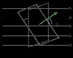
Tension vector flow. Let us place an elementary pad with area . The area must be so small that the electric field strength at all its points can be considered the same. Let's draw a normal to the site (Fig. 1.17). The direction of this normal is chosen arbitrarily. The normal makes an angle with the vector. The flow of the electric field strength vector through a selected surface is the product of the surface area and the projection of the electric field strength vector onto the normal to the area:
 |
where is the projection of the vector onto the normal to the site.
Since the number of field lines piercing a single area is equal to the modulus of the intensity vector in the vicinity of the selected area, the flow of the intensity vector through the surface is proportional to the number of field lines crossing this surface. Therefore, in the general case, the flow of the field strength vector through the area can be visually interpreted as a value equal to the number of field lines penetrating this area:
| . | (1.5) |
Note that the choice of the direction of the normal is conditional; it can be directed in the other direction. Consequently, the flow is an algebraic quantity: the sign of the flow depends not only on the configuration of the field, but also on the relative orientation of the normal vector and the intensity vector. If these two vectors form an acute angle, the flux is positive; if it is obtuse, the flux is negative. In the case of a closed surface, it is customary to take the normal outside the area covered by this surface, that is, to choose the outer normal.
If the field is inhomogeneous and the surface is arbitrary, then the flow is defined as follows. The entire surface must be divided into small elements with area , calculate the stress fluxes through each of these elements, and then sum the fluxes through all elements:
Thus, field strength characterizes the electric field at a point in space. The intensity flow does not depend on the value of the field strength at a given point, but on the distribution of the field over the surface of a particular area.
Electric field lines can only begin on positive charges and end on negative ones. They cannot begin or end in space. Therefore, if there is no electric charge inside a certain closed volume, then the total number of lines entering and exiting this volume must be zero. If more lines leave the volume than enter it, then there is a positive charge inside the volume; if there are more lines coming in than coming out, then there must be a negative charge inside. When the total charge inside the volume is equal to zero or when there is no electric charge in it, the field lines penetrate through it, and the total flux is zero.
These simple considerations do not depend on how the electric charge is distributed within the volume. It can be located in the center of the volume or near the surface that bounds the volume. A volume can contain several positive and negative charges distributed within the volume in any way. Only the total charge determines the total number of incoming or outgoing voltage lines.
As can be seen from (1.4) and (1.5), the flow of the electric field strength vector through an arbitrary closed surface enclosing the charge q, equal to . If inside the surface there is n charges, then, according to the principle of field superposition, the total flux will be the sum of the fluxes of field strengths of all charges and will be equal to , where in this case we mean the algebraic sum of all charges covered by the closed surface.
Gauss's theorem. Gauss was the first to discover the simple fact that the flow of the electric field strength vector through an arbitrary closed surface must be associated with the total charge located inside this volume:
 |
Gauss Karl Friedrich (1777–1855)
Great German mathematician, physicist and astronomer, creator of the absolute system of units in physics. He developed the theory of electrostatic potential and proved the most important theorem of electrostatics (Gauss's theorem). Created a theory for constructing images in complex optical systems. He was one of the first to come to the idea of the possibility of the existence of non-Euclidean geometry. In addition, Gauss made outstanding contributions to almost every branch of mathematics.
The last relation is Gauss's theorem for the electric field: the flux of the intensity vector through an arbitrary closed surface is proportional to the algebraic sum of the charges located inside this surface. The proportionality coefficient depends on the choice of the system of units.
It should be noted that Gauss's theorem is obtained as a consequence of Coulomb's law and the superposition principle. If the electric field strength did not change in inverse proportion to the square of the distance, then the theorem would be invalid. Therefore, Gauss's theorem is applicable to any fields in which the inverse square law and the principle of superposition are strictly satisfied, for example, to the gravitational field. In the case of a gravitational field, the role of charges creating the field is played by the masses of bodies. The flow of gravitational field lines through a closed surface is proportional to the total mass contained within that surface.
Field strength of a charged plane. Let us apply Gauss's theorem to determine the electric field strength of an infinite charged plane. If the plane is infinite and uniformly charged, that is, the surface charge density is the same at any location, then the electric field strength lines at any point are perpendicular to this plane. To show this, we will use the superposition principle for the tension vector. Let us select two elementary sections on the plane, which can be considered point for the point A, in which it is necessary to determine the field strength. As can be seen from Fig. 1.18, the resulting tension vector will be directed perpendicular to the plane. Since the plane can be divided into an infinite number of pairs of such sections for any observation point, it is obvious that the field lines of the charged plane are perpendicular to the plane, and the field is uniform (Fig. 1.19). If this were not so, then when the plane moved along itself, the field at each point in space would change, but this contradicts the symmetry of the charged system (the plane is infinite). In the case of a positively charged plane, the lines of force begin at the plane and end at infinity, while for a negatively charged plane, the lines of force begin at infinity and enter the plane.
 |  |
| Rice. 1.18 | Rice. 1.19 |
To determine the electric field strength of an infinite positively charged plane, we mentally select a cylinder in space, the axis of which is perpendicular to the charged plane, and the bases are parallel to it, and one of the bases passes through the field point of interest to us (Fig. 1.19). The cylinder cuts out an area of area from the charged plane, and the bases of the cylinder, located on different sides of the plane, have the same area.
According to Gauss's theorem, the flow of the electric field strength vector through the surface of the cylinder is related to the electric charge inside the cylinder by the expression:
![]() .
.
Since the stress lines intersect only the bases of the cylinder, the flow through the side surface of the cylinder is zero. Therefore, the flux of the tension vector through the cylindrical surface will consist only of the fluxes through the bases of the cylinder, therefore,
Comparing the last two expressions for the intensity vector flux, we obtain
Electric field strength between oppositely charged plates. If the dimensions of the plates significantly exceed the distance between them, then the electric field of each of the plates can be considered close to the field of an infinite uniformly charged plane. Since the electric field strength lines of oppositely charged plates between the plates are directed in one direction (Fig. 1.20), the field strength between the plates is equal to
![]() .
.
In external space, the electric field strength lines of oppositely charged plates have opposite directions, therefore, outside these plates, the resulting electric field strength is zero. The expression obtained for the intensity is valid for large charged plates, when the intensity is determined at a point located far from their edges.

Electric field strength of a uniformly charged thin wire of infinite length. Let's find the dependence of the electric field strength of a uniformly charged thin wire of infinite length on the distance to the wire axis using Gauss's theorem. Let us select a section of wire of finite length. If the linear charge density on the wire is , then the charge of the selected area is equal to .
Let's consider the field of a point charge $q$ and find the flow of the intensity vector ($\overrightarrow(E)$) through the closed surface $S$. We will assume that the charge is located inside the surface. The flux of the tension vector through any surface is equal to the number of lines of the tension vector that go out (start at the charge, if $q>0$) or the number of lines $\overrightarrow(E)$ going in, if $q \[Ф_E=\frac( q)((\varepsilon )_0)\ \left(1\right),\]
where the sign of the flux coincides with the sign of the charge.
Ostrogradsky-Gauss theorem in integral form
Let us assume that inside the surface S there are N point charges, values $q_1,q_2,\dots q_N.$ From the principle of superposition we know that the resulting field strength of all N charges can be found as the sum of the field strengths that are created by each of the charges, then There is:
Therefore, for the flow of a system of point charges we can write:
Using formula (1), we obtain that:
\[Ф_E=\oint\limits_S(\overrightarrow(E)d\overrightarrow(S))=\frac(1)((\varepsilon )_0)\sum\limits^N_(i=1)(q_i\ )\ left(4\right).\]
Equation (4) means that the flow of the electric field strength vector through a closed surface is equal to the algebraic sum of the charges that are inside this surface, divided by the electric constant. This is the Ostrogradsky-Gauss theorem in integral form. This theorem is a consequence of Coulomb's law. The significance of this theorem is that it allows one to quite simply calculate electric fields for various charge distributions.
As a consequence of the Ostrogradsky-Gauss theorem, it must be said that the flux of the intensity vector ($Ф_E$) through a closed surface in the case in which the charges are outside this surface is equal to zero.
In the case where the discreteness of charges can be ignored, the concept of volumetric charge density ($\rho $) is used if the charge is distributed throughout the volume. It is defined as:
\[\rho =\frac(dq)(dV)\left(5\right),\]
where $dq$ is a charge that can be considered point-like, $dV$ is a small volume. (Regarding $dV$, the following remark must be made. This volume is small enough that the charge density in it can be considered constant, but large enough so that charge discreteness does not begin to appear). The total charge that is in the cavity can be found as:
\[\sum\limits^N_(i=1)(q_i\ )=\int\limits_V(\rho dV)\left(6\right).\]
In this case, we rewrite formula (4) in the form:
\[\oint\limits_S(\overrightarrow(E)d\overrightarrow(S))=\frac(1)((\varepsilon )_0)\int\limits_V(\rho dV)\left(7\right).\ ]
Ostrogradsky-Gauss theorem in differential form
Using the Ostrogradsky-Gauss formula for any field of vector nature, with the help of which the transition from integration over a closed surface to integration over a volume is carried out:
\[\oint\limits_S(\overrightarrow(a)\overrightarrow(dS)=\int\nolimits_V(div))\overrightarrow(a)dV\ \left(8\right),\]
where $\overrightarrow(a)-$field vector (in our case it is $\overrightarrow(E)$), $div\overrightarrow(a)=\overrightarrow(\nabla )\overrightarrow(a)=\frac(\partial a_x)(\partial x)+\frac(\partial a_y)(\partial y)+\frac(\partial a_z)(\partial z)$ -- divergence of the vector $\overrightarrow(a)$ at the point with coordinates ( x,y,z), which maps a vector field to a scalar one. $\overrightarrow(\nabla )=\frac(\partial )(\partial x)\overrightarrow(i)+\frac(\partial )(\partial y)\overrightarrow(j)+\frac(\partial )(\ partial z)\overrightarrow(k)$ - observable operator. (In our case it will be $div\overrightarrow(E)=\overrightarrow(\nabla )\overrightarrow(E)=\frac(\partial E_x)(\partial x)+\frac(\partial E_y)(\partial y) +\frac(\partial E_z)(\partial z)$) -- divergence of the tension vector. Following the above, we rewrite formula (6) as:
\[\oint\limits_S(\overrightarrow(E)\overrightarrow(dS)=\int\nolimits_V(div))\overrightarrow(E)dV=\frac(1)((\varepsilon )_0)\int\limits_V( \rho dV)\left(9\right).\]
The equalities in equation (9) are satisfied for any volume, and this is only feasible if the functions that are in the integrands are equal in each current of space, that is, we can write that:
Expression (10) is the Ostrogradsky-Gauss theorem in differential form. Its interpretation is as follows: charges are sources of an electric field. If $div\overrightarrow(E)>0$, then at these points of the field (charges are positive) we have field sources, if $div\overrightarrow(E)
Assignment: The charge is uniformly distributed over the volume; a cubic surface with side b is selected in this volume. It is inscribed in the sphere. Find the ratio of the tension vector fluxes through these surfaces.
According to Gauss's theorem, the flux ($Ф_E$) of the intensity vector $\overrightarrow(E)$ through a closed surface with a uniform charge distribution over the volume is equal to:
\[Ф_E=\frac(1)((\varepsilon )_0)Q=\frac(1)((\varepsilon )_0)\int\limits_V(\rho dV=\frac(\rho )((\varepsilon ) _0)\int\limits_V(dV)=\frac(\rho V)((\varepsilon )_0))\left(1.1\right).\]
Therefore, we need to determine the volumes of the cube and the ball if the ball is described around this cube. To begin with, the volume of a cube ($V_k$) if its side b is equal to:
Let's find the volume of the ball ($V_(sh)$) using the formula:
where $D$ is the diameter of the ball and (since the ball is circumscribed around the cube), the main diagonal of the cube. Therefore, we need to express the diagonal of a cube in terms of its side. This is easy to do if you use the Pythagorean theorem. To calculate the diagonal of a cube, for example, (1.5), we first need to find the diagonal of the square (the lower base of the cube) (1.6). The length of the diagonal (1.6) is equal to:
In this case, the length of the diagonal (1.5) is equal to:
\[(D=D)_(15)=\sqrt(b^2+((\sqrt(b^2+b^2\ \ \ )))^2)=b\sqrt(3)\ \left (1.5\right).\]
Substituting the found diameter of the ball into (1.3), we obtain:
Now we can find the fluxes of the tension vector through the surface of the cube, it is equal to:
\[Ф_(Ek)=\frac(\rho V_k)((\varepsilon )_0)=\frac(\rho b^3)((\varepsilon )_0)\left(1.7\right),\]
through the surface of the ball:
\[Ф_(Esh)=\frac(\rho V_(sh))((\varepsilon )_0)=\frac(\rho )((\varepsilon )_0)\frac(\sqrt(3))(2) \pi b^3\ \left(1.8\right).\]
Let's find the ratio $\frac(Ф_(Esh))(Ф_(Ek))$:
\[\frac(Ф_(Esh))(Ф_(Ek))=\frac(\frac(с)(\varepsilon_0)\frac(\sqrt(3))(2) \pi b^3)(\frac (сb^3)(\varepsilon_0))=\frac(\pi)(2)\sqrt(3)\ \approx 2.7\left(1.9\right).\]
Answer: The flux through the surface of the ball is 2.7 times greater.
Task: Prove that the charge of a conductor is located on its surface.
We use Gauss's theorem to prove it. Let us select a closed surface of arbitrary shape in the conductor near the surface of the conductor (Fig. 2).

Let us assume that there are charges inside the conductor, we write the Ostrogradsky-Gauss theorem for field divergence for any point on the surface S:
where $\rho is the density\ $of the internal charge. However, there is no field inside the conductor, that is, $\overrightarrow(E)=0$, therefore, $div\overrightarrow(E)=0\to \rho =0$. The Ostrogradsky-Gauss theorem in differential form is local, that is, it is written for a field point, we did not select the point in a special way, therefore, the charge density is zero at any point in the field inside the conductor.
The principle of superposition in combination with Coulomb's law provides the key to calculating the electric field of an arbitrary system of charges, but direct summation of the fields using formula (4.2) usually requires complex calculations. However, in the presence of one or another symmetry of the system of charges, calculations are significantly simplified if we introduce the concept of electric field flow and use Gauss’s theorem.
The concept of electric field flow was introduced into electrodynamics from hydrodynamics. In hydrodynamics, the flow of fluid through a pipe, that is, the volume of fluid N passing through a cross-section of a pipe per unit time, is equal to v ⋅ S, where v is the velocity of the fluid and S is the cross-sectional area of the pipe. If the fluid velocity varies across the cross section, you need to use the integral formula N = ∫ S v → ⋅ d S → . Indeed, let us highlight a small area d S in the velocity field, perpendicular to the velocity vector (Fig. ).
|
The volume of liquid flowing through this area in time d t is equal to v d S d t . If the platform is inclined to the flow, then the corresponding volume will be v d S cos θ d t , where θ is the angle between the velocity vector v → and the normal n → to the platform d S . The volume of liquid flowing through the area d S per unit time is obtained by dividing this value by d t. It is equal to v d S cos θ d t , i.e. scalar product v → ⋅ d S → velocity vector v → by the area element vector d S → = n → d S . The unit vector n → normal to the area d S can be drawn in two directly opposite directions. one of them is conditionally accepted as positive. The normal n → is drawn in this direction. The side of the site from which the normal n → emerges is called external, and the side into which the normal n → enters is called internal. The area element vector d S → is directed along the outer normal n → to the surface, and in magnitude is equal to the area of the element d S = ∣ d S → ∣ . When calculating the volume of fluid flowing through an area S of finite dimensions, it must be developed into infinitesimal areas d S , and then calculate the integral ∫ S v → ⋅ d S → over the entire surface S .
Expressions like ∫ S v → ⋅ d S → are found in many branches of physics and mathematics. They are called the flow of the vector v → through the surface S, regardless of the nature of the vector v →. In electrodynamics the integral
| N = ∫ S E → ⋅ d S → | (5.1) |
Let us assume that the vector E → is represented by a geometric sum
E → = ∑ j E → j .
Multiplying this equality scalarly by d S → and integrating, we obtain
N = ∑ j N j .
where N j is the flow of the vector E → j through the same surface. Thus, from the principle of superposition of electric field strength it follows that the fluxes through the same surface add up algebraically.
Gauss's theorem states that the flux of the vector E → through an arbitrary closed surface is equal to the total charge Q of all particles located inside this surface multiplied by 4 π:
We will carry out the proof of the theorem in three stages.
1. Let's start by calculating the electric field flux of one point charge q (Fig. ). In the simplest case, when the integration surface S is a sphere and the charge is at its center, the validity of Gauss's theorem is almost obvious. On the surface of the sphere, the electric field strength is
E → = q r → ∕ r 3
constant in magnitude and everywhere directed normal to the surface, so that the electric field flux is simply equal to the product E = q ∕ r 2 and the area of the sphere S = 4 π r 2 . Therefore, N = 4 π q. This result is independent of the shape of the surface surrounding the charge. To prove this, we select an arbitrary area of the surface of a sufficiently small size with the direction of the external normal n → set on it. In Fig. one such segment is shown in an exaggeratedly large (for clarity) size.
The flux of the vector E → through this area is equal to d N = E → ⋅ d S → = E cos θ d S ,
where θ is the angle between the direction E → and the outer normal n → to the area d S . Since E = q ∕ r 2 , and d S cos θ ∕ r 2 in absolute value is the element of the solid angle d Ω = d S ∣ cos θ ∣ ∕ r 2 , under which the area d S is visible from the point where the charge is located,
D N = ± q d Ω .
where the plus and minus signs correspond to the cos θ sign, namely: you should take the plus sign if the vector E → makes an acute angle with the direction of the external normal n →, and the minus sign otherwise.
2. Now consider a finite surface S, covering some selected volume V. With respect to this volume, it is always possible to determine which of the two opposite directions of the normal to any element of the surface S should be considered external. The outer normal is directed from volume V outward. Summing up over segments, up to sign we have N = q Ω, where Ω is the solid angle at which the surface S is visible from the point where the charge q is located. If the surface S is closed, then Ω = 4 π, provided that the charge q is inside S. Otherwise Ω = 0. To clarify the last statement, we can again refer to Fig. .
It is obvious that the flows through segments of a closed surface, based on equal solid angles, but facing in opposite directions, cancel each other. It is also obvious that if the charge is outside the closed surface, then for any segment facing outward there is a corresponding segment facing inward.
3. Finally, using the principle of superposition, we arrive at the final formulation of Gauss’s theorem (). Indeed, the field of a system of charges is equal to the sum of the fields of each charge separately, but only charges located inside the closed surface make a non-zero contribution to the right side of the theorem (). This completes the proof.
In macroscopic bodies, the number of charge carriers is so large that it is convenient to represent a discrete ensemble of particles in the form of a continuous distribution, introducing the concept of charge density. By definition, the charge density ρ is the ratio Δ Q ∕ Δ V in the limit when the volume Δ V tends to a physically infinitesimal value:
where the integration on the right side is carried out over the volume V closed by the surface S.Gauss's theorem gives one scalar equation for three components of the vector E →, so this theorem alone is not enough to calculate the electric field. A known symmetry of the charge density distribution is necessary so that the problem can be reduced to a single scalar equation. Gauss's theorem makes it possible to find the field in cases where the surface of integration in () can be chosen so that the electric field strength E is constant over the entire surface. Let's look at the most instructive examples.
▸ Problem 5.1
Find the field of a sphere uniformly charged in volume or surfaces.
Solution: Electric field of a point charge E → = q r → ∕ r 3 tends to infinity at r → 0 . This fact shows the inconsistency of the idea elementary particles by point charges. If the charge q uniformly distributed over the volume of a sphere of finite radius a , then the electric field has no singularities.
From the symmetry of the problem it is clear that the electric field E → everywhere is directed radially, and its tension E = E(r) depends only on the distance r to the center of the ball. Then the electric field flow through a sphere of radius r is simply equal to 4 π r 2 E (Fig. ).
On the other hand, the charge inside the same sphere is equal to the total charge ball Q if r ≥ a. Equating 4 π r 2 E to the charge q of the ball multiplied by 4 π, we obtain: E (r) = q ∕ r 2 .Thus, in external space, a charged ball creates such a field as if all the charge were concentrated at its center. This result is valid for any spherically symmetric charge distribution.
The field inside the ball is E (r) = Q ∕ r 2, where Q is the charge inside the sulfur of radius r. If the charge is uniformly distributed throughout the volume of the ball, then Q = q (r ∕ a) 3 . In this case
E (r) = q r ∕ a 3 = (4 π ∕ 3) ρ r ,
where ρ = q ∕ (4 π a 3 ∕ 3) — charge density. Inside the ball, the field decreases linearly from its maximum values on the surface of the ball to zero at its center (Fig. ).
Function E(r) at the same time, it is finite and continuous everywhere.If the charge is distributed over the surface of the ball, then Q = 0, and therefore also E = 0. This result is also valid for the case when inside a spherical there is no charge cavity, and external charges are distributed spherically symmetrically. ▸ Problem 5.2
Find the field of a uniformly charged infinite thread; thread radius a, charge per unit length ϰ.
▸ Problem 5.3
Find the field of an infinite straight thread and an infinitely long uniformly charged cylinder.
▸ Problem 5.4
Find the field of an infinite charged plane and uniformly charged infinite flat layer.
Solution: Due to the symmetry of the problem, the field is directed normal to the layer and depends only on the distance x from plane of symmetry of the plate. To calculate a field using Gauss's theorem, it is convenient to choose the surface of integration S in in the form of a parallelipiped, as shown in Fig. .
The last result is obtained by passing to the limit a → 0 while simultaneously increasing the charge densityρ so that the value σ = ρ a remained unchanged. On opposite sides of the plane the electric field strength is the same in magnitude, but opposite in direction. Therefore, when passing through charged plane, the field changes abruptly by the amount 4 π σ . Note that the plate can be considered infinite if the distance from is negligible compared to its size. On distances very large compared to the dimensions of the plate, it acts like a point charge, and its field decreases back proportional to the square of the distance.The electrostatic field can be clearly depicted using lines of force (tension lines). Power lines are called curves whose tangents at each point coincide with the tension vector E.
Lines of force are a conventional concept and do not really exist. The field lines of a single negative and single positive charge are shown in Fig. 5 are radial straight lines coming from a positive charge or going to a negative charge.
If the density and direction of the field lines throughout the entire volume of the field remain unchanged, such an electrostatic field is considered homogeneous (the number of lines must be numerically equal to the field strength E).
The number of field lines marked ">dS, perpendicular to them, determines flow of the electrostatic field strength vector:
formula" src="http://hi-edu.ru/e-books/xbook785/files/17-1.gif" border="0" align="absmiddle" alt="- projection of the vector E onto the direction of the normal n to the site dS (Fig. 6).
Accordingly, the flow of vector E through an arbitrary closed surface S
mark">S not only the magnitude, but also the sign of the flow can change:
1) with formula" src="http://hi-edu.ru/e-books/xbook785/files/17-4.gif" border="0" align="absmiddle" alt="
3) when selecting"> Let's find the flow of vector E through a spherical surface S, in the center of which there is a point charge q.
In this case, the mark ">E and n coincide at all points of the spherical surface.
Taking into account the field strength of a point charge, the formula" src="http://hi-edu.ru/e-books/xbook785/files/18-2.gif" border="0" align="absmiddle" alt="(! LANG:we get
formula" src="http://hi-edu.ru/e-books/xbook785/files/Fe.gif" border="0" align="absmiddle" alt="- an algebraic quantity depending on the sign of the charge. For example, when q<0 линии Е направлены к заряду и противоположны направлению внешней нормали n ..gif" border="0" align="absmiddle" alt="around the charge q has an arbitrary shape. Obviously, the surface is marked ">E, as is the surface S. Therefore, the flow of vector E through an arbitrary surface is the formula" src="http://hi-edu.ru/e-books/xbook785/files/Fe.gif" border ="0" align="absmiddle" alt=".
If the charge is located outside the closed surface, then, obviously, how many lines enter the closed area, the same number will leave it. As a result, the flux of vector E will be equal to zero.
If the electric field is created by a system of point charges formula" src="http://hi-edu.ru/e-books/xbook785/files/18-4.gif" border="0" align="absmiddle" alt="
This formula is the mathematical expression of Gauss's theorem: the flow of the electric field strength vector E in a vacuum through an arbitrary closed surface is equal to the algebraic sum of the charges that it covers, divided by formula" src="http://hi-edu.ru/e-books/xbook785/files/18-6.gif" border="0" align="absmiddle" alt="
To complete the description, let us also present Gauss’s theorem in a local form, relying not on integral relations, but on the field parameters at a given point in space. To do this, it is convenient to use the differential operator - vector divergence, -
formula" src="http://hi-edu.ru/e-books/xbook785/files/nabla.gif" border="0" align="absmiddle" alt="(“nabla”) -
formula" src="http://hi-edu.ru/e-books/xbook785/files/19-1.gif" border="0" align="absmiddle" alt="
In mathematical analysis, the Gauss-Ostrogradsky theorem is known: the flow of a vector through a closed surface is equal to the integral of its divergence over the volume limited by this surface -
formula" src="http://hi-edu.ru/e-books/xbook785/files/ro.gif" border="0" align="absmiddle" alt=":
formula" src="http://hi-edu.ru/e-books/xbook785/files/19-4.gif" border="0" align="absmiddle" alt="
This expression is Gauss's theorem in local (differential) form.
Gauss's theorem (2.2) allows us to determine the strengths of various electrostatic fields. Let's look at several examples of the application of Gauss's theorem.
1. Let's calculate E electrostatic field created by a uniformly charged spherical surface.
Let us assume that a spherical surface of radius R carries a uniformly distributed charge q, i.e. surface charge density is the same mark everywhere ">r >R from the center of the sphere, we mentally construct a new spherical surface S, symmetrical to the charged sphere. In accordance with Gauss’s theorem
formula" src="http://hi-edu.ru/e-books/xbook785/files/20-1.gif" border="0" align="absmiddle" alt="
For points located on the surface of a charged sphere of radius R, by analogy we can write:
selection">inside a charged sphere, does not contain electrical charges within itself, so the flux mark">E = 0.
The task of calculating the field strength of a system of electric charges using the principle of superposition of electrostatic fields can be greatly simplified if we apply the theorem discovered by the German scientist K. Gauss (1777-1855), which determines the flow of the electric field strength vector through an arbitrary closed surface.
From the definition of the intensity vector flux through a closed surface, the intensity vector flux through a spherical surface of radius r, which covers a point charge Q located at its center (Fig. 1), is equal to
This result is valid for a closed surface of arbitrary shape. Indeed, if you enclose a sphere (Fig. 1) in an arbitrary closed surface, then each line of tension that penetrates the sphere will also pass through this surface.
If a closed surface of any shape encloses a charge (Fig. 2), then when any tension line intersects with the surface, it either enters or leaves it. When calculating flux, an odd number of intersections ultimately reduces to a single intersection, since the flux is assumed to be positive if lines of tension leave the surface, and negative for lines that enter the surface. If a closed surface does not enclose a charge, then the flux through it is zero, so how the number of tension lines that enter the surface is equal to the number of tension lines that exit it.
This means that for a surface of arbitrary shape, if it is closed and contains a point charge Q, the flow of the vector E will be equal to Q/ε 0, i.e.
The sign of the flux coincides with the sign of the charge Q.
Let us study the general case of an arbitrary surface surrounding n charges. Using the principle of superposition, tension E field, which is created by all charges, is equal to the sum of the intensities E i fields that are created by each charge separately. That's why
According to (1), each of the integrals that appears under the sum sign is equal to Q i /ε 0 . Means,
![]() (2)
(2)
Formula (2) expresses Gauss's theorem for the electrostatic field in vacuum: the flow of the electrostatic field strength vector in a vacuum through an arbitrary closed surface is equal to the algebraic sum of the charges contained inside this surface, divided by ε 0. This theorem was obtained mathematically for a vector field of arbitrary nature by the Russian mathematician M.V. Ostrogradsky (1801-1862), and then independently of him in relation to the electrostatic field - by K. Gauss.
In the general case, electric charges can be distributed with a certain volume density ρ=dQ/dV, which is different in different places in space. Then the total charge contained inside the closed surface S, which covers a certain volume V,
![]() (3)
(3)
Using formula (3), Gauss’s theorem (2) can be written as follows:
Circulation of the voltage vector is the work done by electric forces when moving a single positive charge along a closed path L
| | (13.18) |
Since the work of the electrostatic field forces along a closed loop is zero (the work of the potential field forces), therefore the circulation of the electrostatic field strength along a closed loop is zero.
Electrostatic field potential. The field of a conservative force can be described not only by a vector function, but an equivalent description of this field can be obtained by defining a suitable scalar quantity at each of its points. For an electrostatic field, this quantity is electrostatic field potential, defined as the ratio of the potential energy of the test charge q to the magnitude of this charge, = W P / q, from which it follows that the potential is numerically equal to the potential energy possessed by a unit positive charge at a given point in the field. The unit of measurement for potential is the Volt (1 V).
Point charge field potential Q in a homogeneous isotropic medium with dielectric constant :
Superposition principle. The potential is a scalar function; the principle of superposition is valid for it. So for the field potential of a system of point charges Q 1, Q 2, Qn we have
![]() ,
,
Where r i- distance from the field point with potential to the charge Q i. If the charge is arbitrarily distributed in space, then
![]() ,
,
Where r- distance from the elementary volume d x,d y,d z to point ( x, y, z), where the potential is determined; V- the volume of space in which the charge is distributed.
Potential and work of electric field forces. Based on the definition of potential, it can be shown that the work done by the electric field forces when moving a point charge q from one point of the field to another is equal to the product of the magnitude of this charge and the potential difference at the initial and final points of the path, A = q (
If, by analogy with potential energy, we assume that at points infinitely distant from electric charges - field sources, the potential is zero, then the work of electric field forces when moving a charge q from point 1 to infinity can be represented as A q 1 .
Thus, the potential at a given point of the electrostatic field is physical quantity numerically equal to the work done by the forces of the electric field when moving a unit positive point charge from a given point in the field to an infinitely distant one: = A / q.
In some cases, the electric field potential is more clearly defined as a physical quantity numerically equal to the work of external forces against the forces of the electric field when moving a unit positive point charge from infinity to a given point. It is convenient to write the last definition as follows:
In modern science and technology, especially when describing phenomena occurring in the microcosm, a unit of work and energy called electron-volt(eV). This is the work done when moving a charge equal to the charge of an electron between two points with a potential difference of 1 V: 1 eV = 1.6010 C1 V = 1.6010 J
Equipotential surfaces- a concept applicable to any potential vector field, for example, a static electric field or a Newtonian gravitational field. An equipotential surface is a surface on which the scalar potential of a given potential field takes on a constant value (potential level surface). Another, equivalent, definition is a surface that is orthogonal to the field lines at any point.
The surface of a conductor in electrostatics is an equipotential surface. In addition, placing a conductor on an equipotential surface does not change the configuration of the electrostatic field. This fact is used in the image method, which allows the calculation of the electrostatic field for complex configurations.
In a (stationary) gravitational field, the level of a stationary fluid is established along the equipotential surface. In particular, it can be approximately stated that the level of the oceans passes along the equipotential surface of the Earth’s gravitational field. The shape of the surface of the oceans, extended to the surface of the Earth, is called the geoid and plays an important role in geodesy. The geoid is thus an equipotential surface of gravity, consisting of a gravitational and a centrifugal component.